Adaptive spline fit#
from astropy.io import fits
from astropy.table import QTable
import astropy.units as u
from datetime import datetime
import matplotlib.patches as patches
import matplotlib.pyplot as plt
import numpy as np
import os
import requests
import teareduce as tea
time_ini = datetime.now()
Download the required files
for fname in [
    'notebooks/adaptivespl/response_data_BD33d2642_G100.fits',
    'notebooks/adaptivespl/skycalc_transmission_R20000_400-800nm.txt'
]:
    tea.get_cookbook_file(fname)
File response_data_BD33d2642_G100.fits already exists locally. Skipping download.
File skycalc_transmission_R20000_400-800nm.txt already exists locally. Skipping download.
There are many situations in which it is useful to perform a smooth fit to a series of points, but a polynomial fit does not provide the necessary flexibility. In such cases, spline fitting is often used. To facilitate this task, teareduce provides a class, named AdaptiveLSQUnivariateSpline that allows performing this type of fit without having to predefine the locations of the knots (the points where the different polynomial segments join to create a continuous and smooth curve), requiring only the specification of the number of intermediate knots to use.
The AdaptiveLSQUnivariateSpline inherits from LSQUnivariateSpline from the scipy package, introducing two new parameters:
adaptive(bool): if True, optimize the knot location numericallytolerance(float): value to be employed in the minimisation process
The numerical minimisation procedure is carried out with the help of the lmfit package, following the procedure described in Cardiel (2009).
help(tea.AdaptiveLSQUnivariateSpline)
Help on class AdaptiveLSQUnivariateSpline in module teareduce.numsplines:

class AdaptiveLSQUnivariateSpline(scipy.interpolate._fitpack2.LSQUnivariateSpline)
 |  AdaptiveLSQUnivariateSpline(
 |      x,
 |      y,
 |      t,
 |      w=None,
 |      bbox=(None, None),
 |      k=3,
 |      ext=0,
 |      check_finite=False,
 |      adaptive=True,
 |      tolerance=1e-07
 |  )
 |
 |  Extend scipy.interpolate.LSQUnivariateSpline.
 |
 |  One-dimensional spline with explicit internal knots.
 |
 |  This is actually a wrapper of
 |  `scipy.interpolate.LSQUnivariateSpline`
 |  with the addition of using adaptive knot location determined
 |  numerically (after normalising the x and y arrays before
 |  the minimisation process).
 |
 |  Parameters
 |  ----------
 |  x : (N,) array_like
 |      Input dimension of data points -- must be increasing
 |  y : (N,) array_like
 |      Input dimension of data points
 |  t : (M,) array_like or int
 |      When integer it indicates the number of equidistant
 |      interior knots. When array_like it provides the location
 |      of the interior knots of the spline; must be in ascending
 |      order and::
 |
 |       bbox[0] < t[0] < ... < t[-1] < bbox[-1]
 |
 |  w : (N,) array_like, optional
 |      weights for spline fitting.  Must be positive.
 |      If None (default), weights are all equal.
 |  bbox : (2,) array_like, optional
 |      2-sequence specifying the boundary of the approximation
 |      interval. If None (default), ``bbox = [x[0], x[-1]]``.
 |  k : int, optional
 |      Degree of the smoothing spline.  Must be 1 <= `k` <= 5.
 |      Default is k=3, a cubic spline.
 |  ext : int or str, optional
 |      Controls the extrapolation mode for elements
 |      not in the interval defined by the knot sequence.
 |
 |      * if ext=0 or 'extrapolate', return the extrapolated value.
 |      * if ext=1 or 'zeros', return 0
 |      * if ext=2 or 'raise', raise a ValueError
 |      * if ext=3 of 'const', return the boundary value.
 |
 |      The default value is 0.
 |
 |  check_finite : bool, optional
 |      Whether to check that the input arrays contain only finite
 |      numbers, that the x array is increasing and that the
 |      x and y arrays are 1-D and with the same length.
 |      Disabling may give a performance gain, but may
 |      result in problems (crashes, non-termination or non-sensical
 |      results) if the inputs do contain infinities or NaNs.
 |      Default is True.
 |  adaptive : bool, optional
 |      Whether to optimise knot location following the procedure
 |      described in Cardiel (2009); see:
 |      http://cdsads.u-strasbg.fr/abs/2009MNRAS.396..680C
 |      Default is True.
 |  tolerance : float, optional
 |      Tolerance for Nelder-Mead minimisation process.
 |
 |  Attributes
 |  ----------
 |  _params : instance of Parameters()
 |      Initial parameters before minimisation.
 |  _result : Minimizer output
 |      Result of the minimisation process.
 |
 |  See also
 |  --------
 |  LSQUnivariateSpline : Superclass
 |
 |  Method resolution order:
 |      AdaptiveLSQUnivariateSpline
 |      scipy.interpolate._fitpack2.LSQUnivariateSpline
 |      scipy.interpolate._fitpack2.UnivariateSpline
 |      builtins.object
 |
 |  Methods defined here:
 |
 |  __init__(
 |      self,
 |      x,
 |      y,
 |      t,
 |      w=None,
 |      bbox=(None, None),
 |      k=3,
 |      ext=0,
 |      check_finite=False,
 |      adaptive=True,
 |      tolerance=1e-07
 |  )
 |      One-dimensional spline with explicit internal knots.
 |
 |  get_params(self)
 |      Return initial parameters for minimisation process.
 |
 |  get_result(self)
 |      Return result of minimisation process.
 |
 |  ----------------------------------------------------------------------
 |  Methods inherited from scipy.interpolate._fitpack2.UnivariateSpline:
 |
 |  __call__(self, x, nu=0, ext=None)
 |      Evaluate spline (or its nu-th derivative) at positions x.
 |
 |      Parameters
 |      ----------
 |      x : array_like
 |          A 1-D array of points at which to return the value of the smoothed
 |          spline or its derivatives. Note: `x` can be unordered but the
 |          evaluation is more efficient if `x` is (partially) ordered.
 |      nu  : int
 |          The order of derivative of the spline to compute.
 |      ext : int
 |          Controls the value returned for elements of `x` not in the
 |          interval defined by the knot sequence.
 |
 |          * if ext=0 or 'extrapolate', return the extrapolated value.
 |          * if ext=1 or 'zeros', return 0
 |          * if ext=2 or 'raise', raise a ValueError
 |          * if ext=3 or 'const', return the boundary value.
 |
 |          The default value is 0, passed from the initialization of
 |          UnivariateSpline.
 |
 |  antiderivative(self, n=1)
 |      Construct a new spline representing the antiderivative of this spline.
 |
 |      Parameters
 |      ----------
 |      n : int, optional
 |          Order of antiderivative to evaluate. Default: 1
 |
 |      Returns
 |      -------
 |      spline : UnivariateSpline
 |          Spline of order k2=k+n representing the antiderivative of this
 |          spline.
 |
 |      Notes
 |      -----
 |
 |      .. versionadded:: 0.13.0
 |
 |      See Also
 |      --------
 |      splantider, derivative
 |
 |      Examples
 |      --------
 |      >>> import numpy as np
 |      >>> from scipy.interpolate import UnivariateSpline
 |      >>> x = np.linspace(0, np.pi/2, 70)
 |      >>> y = 1 / np.sqrt(1 - 0.8*np.sin(x)**2)
 |      >>> spl = UnivariateSpline(x, y, s=0)
 |
 |      The derivative is the inverse operation of the antiderivative,
 |      although some floating point error accumulates:
 |
 |      >>> spl(1.7), spl.antiderivative().derivative()(1.7)
 |      (array(2.1565429877197317), array(2.1565429877201865))
 |
 |      Antiderivative can be used to evaluate definite integrals:
 |
 |      >>> ispl = spl.antiderivative()
 |      >>> ispl(np.pi/2) - ispl(0)
 |      2.2572053588768486
 |
 |      This is indeed an approximation to the complete elliptic integral
 |      :math:`K(m) = \int_0^{\pi/2} [1 - m\sin^2 x]^{-1/2} dx`:
 |
 |      >>> from scipy.special import ellipk
 |      >>> ellipk(0.8)
 |      2.2572053268208538
 |
 |  derivative(self, n=1)
 |      Construct a new spline representing the derivative of this spline.
 |
 |      Parameters
 |      ----------
 |      n : int, optional
 |          Order of derivative to evaluate. Default: 1
 |
 |      Returns
 |      -------
 |      spline : UnivariateSpline
 |          Spline of order k2=k-n representing the derivative of this
 |          spline.
 |
 |      See Also
 |      --------
 |      splder, antiderivative
 |
 |      Notes
 |      -----
 |
 |      .. versionadded:: 0.13.0
 |
 |      Examples
 |      --------
 |      This can be used for finding maxima of a curve:
 |
 |      >>> import numpy as np
 |      >>> from scipy.interpolate import UnivariateSpline
 |      >>> x = np.linspace(0, 10, 70)
 |      >>> y = np.sin(x)
 |      >>> spl = UnivariateSpline(x, y, k=4, s=0)
 |
 |      Now, differentiate the spline and find the zeros of the
 |      derivative. (NB: `sproot` only works for order 3 splines, so we
 |      fit an order 4 spline):
 |
 |      >>> spl.derivative().roots() / np.pi
 |      array([ 0.50000001,  1.5       ,  2.49999998])
 |
 |      This agrees well with roots :math:`\pi/2 + n\pi` of
 |      :math:`\cos(x) = \sin'(x)`.
 |
 |  derivatives(self, x)
 |      Return all derivatives of the spline at the point x.
 |
 |      Parameters
 |      ----------
 |      x : float
 |          The point to evaluate the derivatives at.
 |
 |      Returns
 |      -------
 |      der : ndarray, shape(k+1,)
 |          Derivatives of the orders 0 to k.
 |
 |      Examples
 |      --------
 |      >>> import numpy as np
 |      >>> from scipy.interpolate import UnivariateSpline
 |      >>> x = np.linspace(0, 3, 11)
 |      >>> y = x**2
 |      >>> spl = UnivariateSpline(x, y)
 |      >>> spl.derivatives(1.5)
 |      array([2.25, 3.0, 2.0, 0])
 |
 |  get_coeffs(self)
 |      Return spline coefficients.
 |
 |  get_knots(self)
 |      Return positions of interior knots of the spline.
 |
 |      Internally, the knot vector contains ``2*k`` additional boundary knots.
 |
 |  get_residual(self)
 |      Return weighted sum of squared residuals of the spline approximation.
 |
 |      This is equivalent to::
 |
 |           sum((w[i] * (y[i]-spl(x[i])))**2, axis=0)
 |
 |  integral(self, a, b)
 |      Return definite integral of the spline between two given points.
 |
 |      Parameters
 |      ----------
 |      a : float
 |          Lower limit of integration.
 |      b : float
 |          Upper limit of integration.
 |
 |      Returns
 |      -------
 |      integral : float
 |          The value of the definite integral of the spline between limits.
 |
 |      Examples
 |      --------
 |      >>> import numpy as np
 |      >>> from scipy.interpolate import UnivariateSpline
 |      >>> x = np.linspace(0, 3, 11)
 |      >>> y = x**2
 |      >>> spl = UnivariateSpline(x, y)
 |      >>> spl.integral(0, 3)
 |      9.0
 |
 |      which agrees with :math:`\int x^2 dx = x^3 / 3` between the limits
 |      of 0 and 3.
 |
 |      A caveat is that this routine assumes the spline to be zero outside of
 |      the data limits:
 |
 |      >>> spl.integral(-1, 4)
 |      9.0
 |      >>> spl.integral(-1, 0)
 |      0.0
 |
 |  roots(self)
 |      Return the zeros of the spline.
 |
 |      Notes
 |      -----
 |      Restriction: only cubic splines are supported by FITPACK. For non-cubic
 |      splines, use `PPoly.root` (see below for an example).
 |
 |      Examples
 |      --------
 |
 |      For some data, this method may miss a root. This happens when one of
 |      the spline knots (which FITPACK places automatically) happens to
 |      coincide with the true root. A workaround is to convert to `PPoly`,
 |      which uses a different root-finding algorithm.
 |
 |      For example,
 |
 |      >>> x = [1.96, 1.97, 1.98, 1.99, 2.00, 2.01, 2.02, 2.03, 2.04, 2.05]
 |      >>> y = [-6.365470e-03, -4.790580e-03, -3.204320e-03, -1.607270e-03,
 |      ...      4.440892e-16,  1.616930e-03,  3.243000e-03,  4.877670e-03,
 |      ...      6.520430e-03,  8.170770e-03]
 |      >>> from scipy.interpolate import UnivariateSpline
 |      >>> spl = UnivariateSpline(x, y, s=0)
 |      >>> spl.roots()
 |      array([], dtype=float64)
 |
 |      Converting to a PPoly object does find the roots at `x=2`:
 |
 |      >>> from scipy.interpolate import splrep, PPoly
 |      >>> tck = splrep(x, y, s=0)
 |      >>> ppoly = PPoly.from_spline(tck)
 |      >>> ppoly.roots(extrapolate=False)
 |      array([2.])
 |
 |      See Also
 |      --------
 |      sproot
 |      PPoly.roots
 |
 |  set_smoothing_factor(self, s)
 |      Continue spline computation with the given smoothing
 |      factor s and with the knots found at the last call.
 |
 |      This routine modifies the spline in place.
 |
 |  ----------------------------------------------------------------------
 |  Static methods inherited from scipy.interpolate._fitpack2.UnivariateSpline:
 |
 |  validate_input(x, y, w, bbox, k, s, ext, check_finite)
 |
 |  ----------------------------------------------------------------------
 |  Data descriptors inherited from scipy.interpolate._fitpack2.UnivariateSpline:
 |
 |  __dict__
 |      dictionary for instance variables
 |
 |  __weakref__
 |      list of weak references to the object
Example: computation of response curve#
Read input data
input_file = 'response_data_BD33d2642_G100.fits'

with fits.open(input_file) as hdul:
    hdul.info()
    header = hdul[1].header
Filename: response_data_BD33d2642_G100.fits
No.    Name      Ver    Type      Cards   Dimensions   Format
  0  PRIMARY       1 PrimaryHDU       9   ()
  1                1 BinTableHDU     14   2048R x 2C   [D, D]
The first FITS extension contains a binary table with the initial response curve obtained
The first extension contains a binary table with the initial response curve, calculated as the ratio between the observed spectrum (in \({\rm ADU}/{\rm s}\)) and the tabulated spectrum (in \({\rm erg}\,{\rm cm}^{-2}\,{\rm s}^{-1}\,\unicode{x212B}^{-1}\)).
header
XTENSION= 'BINTABLE'           / binary table extension
BITPIX  =                    8 / array data type
NAXIS   =                    2 / number of array dimensions
NAXIS1  =                   16 / length of dimension 1
NAXIS2  =                 2048 / length of dimension 2
PCOUNT  =                    0 / number of group parameters
GCOUNT  =                    1 / number of groups
TFIELDS =                    2 / number of table fields
TTYPE1  = 'wavelength'
TFORM1  = 'D       '
TUNIT1  = 'Angstrom'
TTYPE2  = 'response_data'
TFORM2  = 'D       '
TUNIT2  = 'ADU/s/FLAM'
response_data = QTable.read(input_file, hdu=1)
WARNING: UnitsWarning: 'ADU/s/FLAM' did not parse as fits unit: At col 0, Unit 'ADU' not supported by the FITS standard. Did you mean AU or adu? If this is meant to be a custom unit, define it with 'u.def_unit'. To have it recognized inside a file reader or other code, enable it with 'u.add_enabled_units'. For details, see https://docs.astropy.org/en/latest/units/combining_and_defining.html [astropy.units.core]
We received a warning because the units 'ADU/s/FLAM' in the second column of the table are not part of the FITS standard. To avoid problems in the code we will use next, we redefine this expression using valid units.
response_units = u.def_unit('ADU/s/FLAM')
response_data
| wavelength | response_data |
|---|---|
| Angstrom | ADU/s/FLAM |
| float64 | float64 |
| 4220.0 | 39427588791206.695 |
| 4222.0 | 39714436792249.06 |
| 4224.0 | 39784267391699.305 |
| 4226.0 | 40587338329114.48 |
| 4228.0 | 40123370683430.62 |
| 4230.0 | 42073303260572.02 |
| 4232.0 | 41331589582946.73 |
| 4234.0 | 41229670352075.2 |
| 4236.0 | 41948512903698.836 |
| ... | ... |
| 8298.0 | 129111894057217.53 |
| 8300.0 | 129530065711286.72 |
| 8302.0 | 142369449268286.38 |
| 8304.0 | 134472112423705.3 |
| 8306.0 | 135941949777498.97 |
| 8308.0 | 132715306899843.95 |
| 8310.0 | 139485355521601.33 |
| 8312.0 | 137408614652947.81 |
| 8314.0 | 138341505029212.25 |
We also read an ASCII file containing information on the transmission of the Earth’s atmosphere.
telluric_tabulated = np.genfromtxt('skycalc_transmission_R20000_400-800nm.txt')
telluric_tabulated
array([[4.00007171e+02, 7.33015000e-01],
       [4.00027172e+02, 7.33056000e-01],
       [4.00047174e+02, 7.33099000e-01],
       ...,
       [8.99898946e+02, 9.74310000e-01],
       [8.99943942e+02, 9.73631000e-01],
       [8.99988940e+02, 9.73231000e-01]], shape=(16219, 2))
Prepare the data to be displayed
# response data
wavelength = response_data['wavelength']
response = response_data['response_data']

# transmission data
xtelluric = telluric_tabulated[:,0] * 10  # convert from nm to Angstrom
ytelluric = telluric_tabulated[:,1]
# extract data in the required wavelength range
iok = np.argwhere(np.logical_and(xtelluric >= wavelength.value.min(), xtelluric <= wavelength.value.max()))
xtelluric = xtelluric[iok]
ytelluric = ytelluric[iok]
# normalize data
ytelluric = ytelluric / ytelluric.max()
Define functions to plot data and legend (in this way we avoid repeating code)
def plot_data(ax1):
    ax1.plot(wavelength, response, label='response curve')
    ax1.set_xlabel(f'Wavelength ({wavelength.unit})')
    if str(response.unit) != 'ADU/s/FLAM':
        raise ValueError(f'unexpected response units: {str(response.unit)}')
    ax1.set_ylabel(r'Response (ADU/s) / (${\rm erg}\;{\rm cm}^{−2}\; {\rm s}^{−1}\;{\rm\AA}^{−1}$)')
    ax1.set_title(input_file)

    ax2 = ax1.twinx()
    ax2.plot(xtelluric, ytelluric, color='C2', label='telluric lines', alpha=0.5)
    ax2.set_ylabel('relative atmosphere transmission', color='C2')
    ax2.set_xlim(wavelength.value.min(), wavelength.value.max())

    return ax2

def display_legend(ax1, ax2):
    # merge labels
    handles1, labels1 = ax1.get_legend_handles_labels()
    handles2, labels2 = ax2.get_legend_handles_labels()
    for handle, label in zip(handles2, labels2):
        handles1.append(handle)
        labels1.append(label)
    ax1.legend(handles1, labels1, loc=2)
Display the data
fig, ax1 = plt.subplots(figsize=(10, 5))

ax2 = plot_data(ax1)
display_legend(ax1, ax2)

plt.tight_layout()
plt.show()
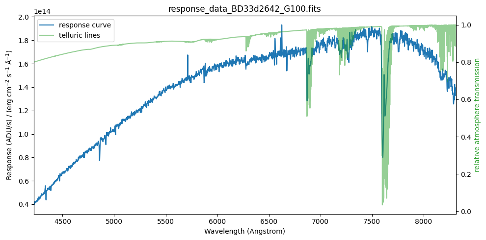
The previous graph shows the relative transmission of the atmosphere (green curve), which provides a very good explanation for the observed telluric lines. Note that we know the atmospheric transmission with very high spectral resolution, significantly higher than the spectral resolution of our observed spectrum. In principle, we would need to convolve the relative atmospheric transmission (for example, with a Gaussian kernel) in order to better reproduce the telluric absorptions. However, it is not worthwhile to spend time on this. Telluric absorptions also depend on the airmass, and correcting these regions of spectra is a formidable challenge; in this example we are simply going to ignore these regions of the spectra.
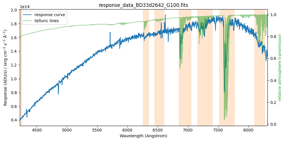
The response curve we will use will be a smooth fit to the resulting spectrum. But before performing the fit, we will remove problematic regions (particularly those affected by telluric absorptions). We define these regions as intervals in wavelength (Ångström).
# wavelength ranges
list_bad_regions = [
    (4200, 4250),
    (6260, 6350),
    (6450, 6600),
    (6850, 7050),
    (7160, 7400),
    (7520, 7770),
    (8100, 8270),
]
Auxiliary function to plot the problematic telluric windows.
def plot_telluric_windows(ax1):
    ymin, ymax = ax1.get_ylim()
    height = ymax - ymin
    for w1, w2 in list_bad_regions:
        width = w2 - w1
        rect = patches.Rectangle(xy=(w1, ymin),
                                 width=width, height=height,
                                 color='C1', alpha=0.2)
        ax1.add_patch(rect)
Repeat plot overplotting the telluric windows
fig, ax1 = plt.subplots(figsize=(10, 5))

ax2 = plot_data(ax1)
display_legend(ax1, ax2)
plot_telluric_windows(ax1)

plt.tight_layout()
plt.show()
We assign a very small weight to the spectral data points corresponding to the problematic regions (weight_bad_region = 0.001; the weight of a normal point will be 1.0). Note that we keep these points nonetheless, so that the fit is computed over the entire spectral range.
naxis1 = len(wavelength)

weight = np.ones((naxis1))
weight_bad_region = 0.001

for w1, w2 in list_bad_regions:
    i1 = (np.abs(wavelength.value - w1)).argmin()
    i2 = (np.abs(wavelength.value - w2)).argmin()
    weight[i1:(i2+1)] = weight_bad_region
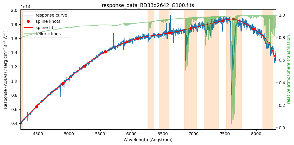
We perform a fit using an adaptive spline (spline fit with movable knots). By trial and error we find that 11 intermediate knots work well.
number_of_intermediate_knots = 11

spl = tea.AdaptiveLSQUnivariateSpline(x=wavelength.value, y=response.value, w=weight,
                                      t=number_of_intermediate_knots)
Evaluate fit and determine location of knots.
response_curve = spl(wavelength.value) * response_units

xknots = spl.get_knots()
yknots = spl(xknots)
Display data and fit (with knots)
fig, ax1 = plt.subplots(figsize=(10, 5))

ax2 = plot_data(ax1)
ax1.plot(xknots, yknots, 'ro', label='spline knots')
ax1.plot(wavelength, response_curve, 'r-', label='spline fit')
display_legend(ax1, ax2)
plot_telluric_windows(ax1)

plt.tight_layout()
plt.show()
tea.elapsed_time_since(time_ini)
system...........: Darwin
release..........: 25.2.0
machine..........: arm64
node.............: iblax.fis.ucm.es
Python executable: /Users/cardiel/venv_tea/bin/python3.13
teareduce version: 0.7.1
Initial time.....: 2026-02-06 10:28:20.485048
Final time.......: 2026-02-06 10:28:21.594042
Elapsed time.....: 0:00:01.108994