C distortion and wavelength calibration#
This notebook describes how to perform the C distortion correction and the wavelength calibration of an image following the strategy outlined below.
Important: it is assumed that the data array is oriented such that the spectral direction corresponds to the horizontal axis and the spatial direction to the vertical axis. Additionally, it is assumed that the spectral scale increases from left to right.
Modus operandi:
Identification of lines with known wavelengths: this is done on an average spectrum of the image.
Wavelength calibration of an initial spectrum: this helps determine the appropriate degree of the polynomial to be fitted.
Automatic search for the lines of interest across the entire image (it is possible to skip regions in the spatial direction if necessary).
C distortion fitting: the distortion of each line is fitted using a polynomial of the required degree.
Determination of the wavelength calibration polynomial for each spectrum. This calculation is based on the positions of the lines predicted by the polynomials that describe the C distortion of the image.
Storage of the wavelength calibration polynomials in an auxiliary FITS file.
Application of the wavelength calibration polynomials to perform, in a single step, both the C distortion correction and the wavelength calibration (i.e., transformation of the image to a linear wavelength scale).
from astropy.io import fits
from astropy.nddata import CCDData
import astropy.units as u
from datetime import datetime
import matplotlib.pyplot as plt
from mpl_toolkits.axes_grid1 import make_axes_locatable
import numpy as np
from pathlib import Path
import teareduce as tea
time_ini = datetime.now()
print(time_ini)
2026-02-06 10:27:24.925880
Download the required file
tea.get_cookbook_file('notebooks/wavecalib/ftdz_45324.fits')
File ftdz_45324.fits already exists locally. Skipping download.
tea.avoid_astropy_warnings(True)
We will work with a specific image from Practice 3: ftdz_45324.fits (in this image we have already subtracted the BIAS and DARK, cropped the under and overscan regions, and applied the Flat Field).
input_filename = 'ftdz_45324.fits'
data = fits.getdata(input_filename)
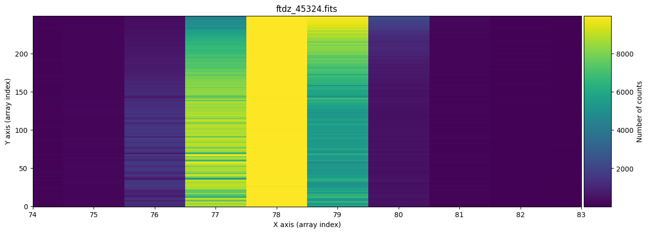
We display the full image and a zoom around one of the lines, which allows us to observe that there is a certain C distortion.
for iplot in range(2):
    if iplot == 0:
        vmin, vmax = np.percentile(data, [5, 95])
    else:
        vmin, vmax = np.percentile(data, [5, 99])
    fig, ax = plt.subplots(figsize=(15, 5))
    tea.imshow(fig, ax, data, vmin=vmin, vmax=vmax, title=f'{input_filename}',
               aspect='auto')
    if iplot == 1:
        ax.set_xlim([74, 83])
    plt.show()
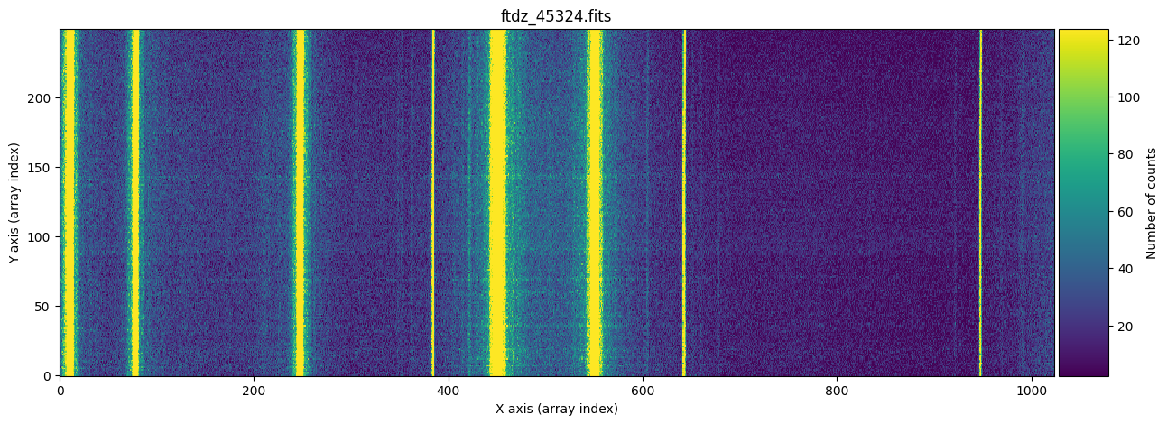
naxis2, naxis1 = data.shape
print(f'NAXIS1, NAXIS2: {naxis1}, {naxis2}')
NAXIS1, NAXIS2: 1024, 250
Automatic search for lines of interest across the entire image.#
We create an instance of type TeaWaveCalibration which, by default, has predefined initial values to carry out the work of calibration and correction of C distortion and wavelength calibration. These initial parameters can be modified as we, through trial and error, find more suitable values for calibrating the image at hand.
wavecalib = tea.TeaWaveCalibration()
wavecalib
TeaWaveCalibration(
    ns_window=11,
    threshold=0,
    sigma_smooth=0,
    nx_window=5,
    delta_flux=0,
    method='gaussian',
    degree_cdistortion=1,
    degree_wavecalib=1,
    peak_wavelengths=None,
    _nlines_reference=None,
    _naxis1=None,
    _naxis2=None,
    _xpeaks_all_lines_array=None,
    _valid_scans=None,
    _list_poly_cdistortion=None,
    _array_poly_wav=None,
    _array_poly_pix=None,
    _array_residual_std_wav=None,
    _array_residual_std_pix=None,
    _array_crval1_linear=None,
    _array_cdelt1_linear=None,
    _array_crmax1_linear=None
)
We can easily view the documentation of the class.
print(tea.TeaWaveCalibration.__doc__)
Auxiliary class to compute and apply wavelength calibration.

It is assumed that the wavelength and spatial directions correspond
to the X (array columns) and Y (array rows) axes, respectively.

Attributes
----------
ns_window : int
    Number of spectra to be (median) averaged. It must be odd.
threshold : float
    Minimum signal to search for peaks.
sigma_smooth : int
    Standard deviation for Gaussian kernel to smooth median spectrum.
    A value of 0 means that no smoothing is performed.
nx_window : int
    Number of pixels (spectral direction) of the window where the
    peaks are sought. It must be odd.
delta_flux : float
    Minimum difference between the flux at the line center and the
    flux at the borders of the window where the peaks are sought.
method : str
    Function to be employed when fitting line peaks:
    - "poly2" : fit to a 2nd order polynomial
    - "gaussian" : fit to a Gaussian
degree_cdistortion : int
    Polynomial degree to fit curvature of each arc line.
degree_wavecalib : int
    Polynomial degree to fit wavelength variation with pixel number.
peak_wavelengths : astropy.unit.Quantity or None
    Array providing the wavelengths of the line peaks, with units.
The first thing we need to do is obtain an approximate position of the line peaks. If there is significant C distortion, it is not advisable to combine many spectra, as this would broaden the lines. On the other hand, it is worth combining several spectra because this improves the signal-to-noise ratio and helps eliminate cosmic rays (if they haven’t already been removed). This is possible because the average spectrum we will work with is obtained using a median average (instead of a mean).
The default parameters we can adjust are:
ns_window: number of spectra that can be collapsed to obtain an average spectrum in which to search for peaks.threshold: minimum number of counts a peak must have to be considered as such.sigma_smooth: for noisy spectra, it is useful to convolve with a Gaussian filter. This parameter indicates the width of that kernel (see usage example below).nx_window: each peak must meet the condition that the central value is the highest within a window of this width. Additionally, the pixels to the right and left of the peak must decrease monotonically. It must be an odd number so that there arenx_window/2pixels on each side of the central peak.delta_flux: within each peak search window (of widthnx_window), the signal at the peak must exceed the value at the pixels located at the edges of the interval by a minimum amount given by thisdelta_fluxfactor. By default, this value is zero. This parameter helps detect/ignore peaks when the arc to be calibrated has a variable continuum signal along the spectral direction, which makes it difficult to find athresholdvalue that works across the entire interval.method: method used to refine the peak position. Only two options are available:poly2orgaussian(a parabola or a Gaussian).degree_cdistortion: degree of the polynomial used to fit the C distortion of the lines.degree_wavecal: degree of the polynomial used for wavelength calibration.
In this example, we will collapse 11 spectra, starting from 120 and ending at 130 (following the FITS numbering convention, which starts at 1). To do this, we use the auxiliary class SliceRegion1D, which allows us to define an interval using either the FITS or Python convention.
ns_range = tea.SliceRegion1D(np.s_[120:130], mode='fits')
ns_range_bis = tea.SliceRegion1D(np.s_[119:130], mode='python')

# check that both instances correspond to the same region
ns_range == ns_range_bis
True
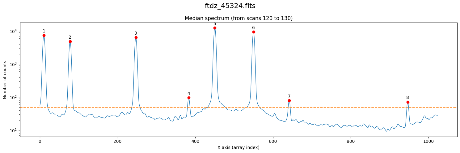
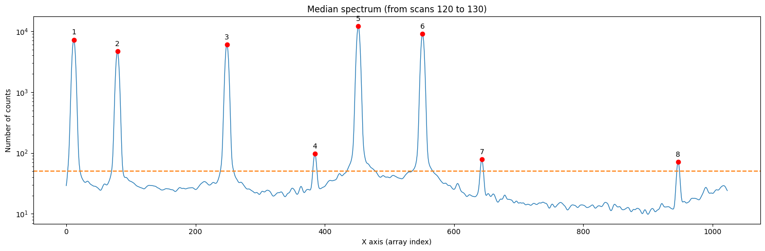
We use the method compute_xpeaks_reference(), which returns an array with the positions of the peaks (in array coordinates; that is, starting from 0), both in real format xpeaks_reference (the positions have been fitted to a Gaussian because method='gaussian' is set in the default parameters) and in integer format ixpeaks_reference (array indices). We also obtain the average spectrum used: spectrum_reference.
xpeaks_reference, ixpeaks_reference, spectrum_reference = wavecalib.compute_xpeaks_reference(
    data=data,
    ns_range=ns_range,
    plot_spectrum=True,
    title=input_filename
)
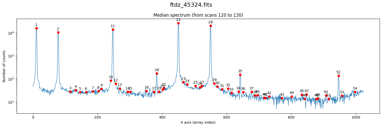
Note that in the representation we are using a logarithmic scale on the vertical axis. In the case of arcs, this is very useful because we often encounter both bright and faint lines.
We have found too many peaks because the default threshold is zero.
xpeaks_reference, ixpeaks_reference, spectrum_reference = wavecalib.compute_xpeaks_reference(
    data=data,
    ns_range=ns_range,
    threshold=50,
    plot_spectrum=True,
    title=input_filename
)
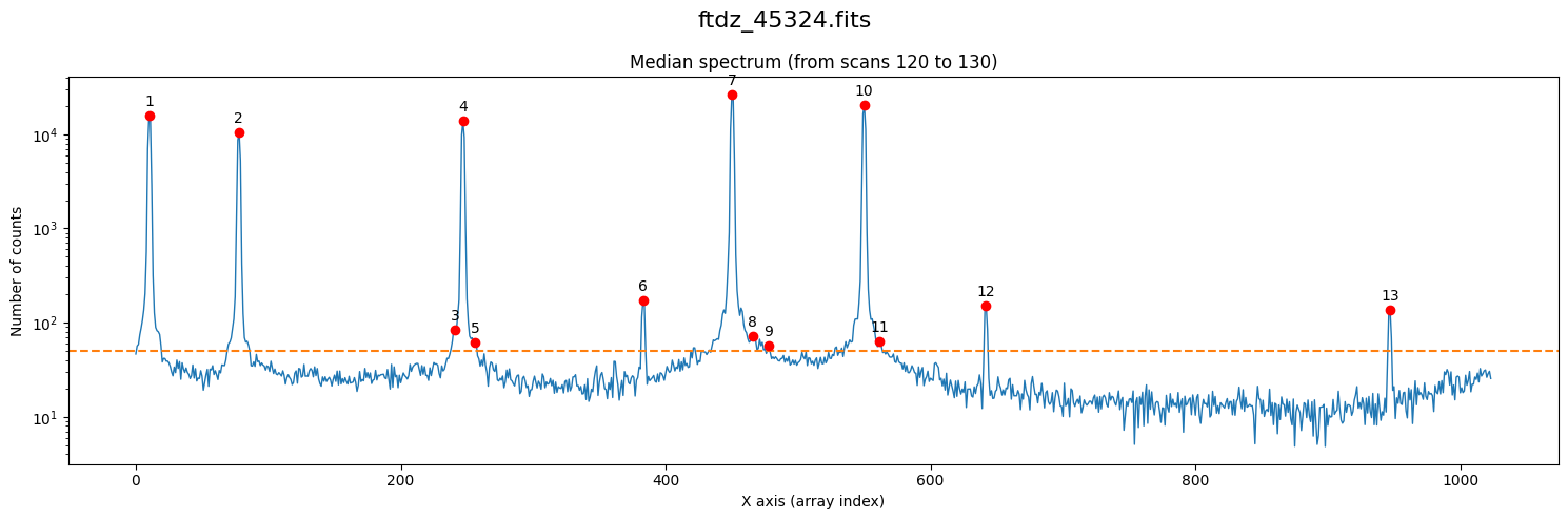
By having modified the threshold parameter, its value has changed in the wavecalib object’s attribute.
wavecalib
TeaWaveCalibration(
    ns_window=11,
    threshold=50,
    sigma_smooth=0,
    nx_window=5,
    delta_flux=0,
    method='gaussian',
    degree_cdistortion=1,
    degree_wavecalib=1,
    peak_wavelengths=None,
    _nlines_reference=None,
    _naxis1=1024,
    _naxis2=250,
    _xpeaks_all_lines_array=None,
    _valid_scans=None,
    _list_poly_cdistortion=None,
    _array_poly_wav=None,
    _array_poly_pix=None,
    _array_residual_std_wav=None,
    _array_residual_std_pix=None,
    _array_crval1_linear=None,
    _array_cdelt1_linear=None,
    _array_crmax1_linear=None
)
We display the individual fit to each of the peaks using the parameter plot_peaks=True (there’s no need to specify the threshold anymore because it will use the current default, which is already 50).
xpeaks_reference, ixpeaks_reference, spectrum_reference = wavecalib.compute_xpeaks_reference(
    data=data,
    ns_range=ns_range,
    plot_spectrum=True,
    plot_peaks=True,
    title=input_filename,
)
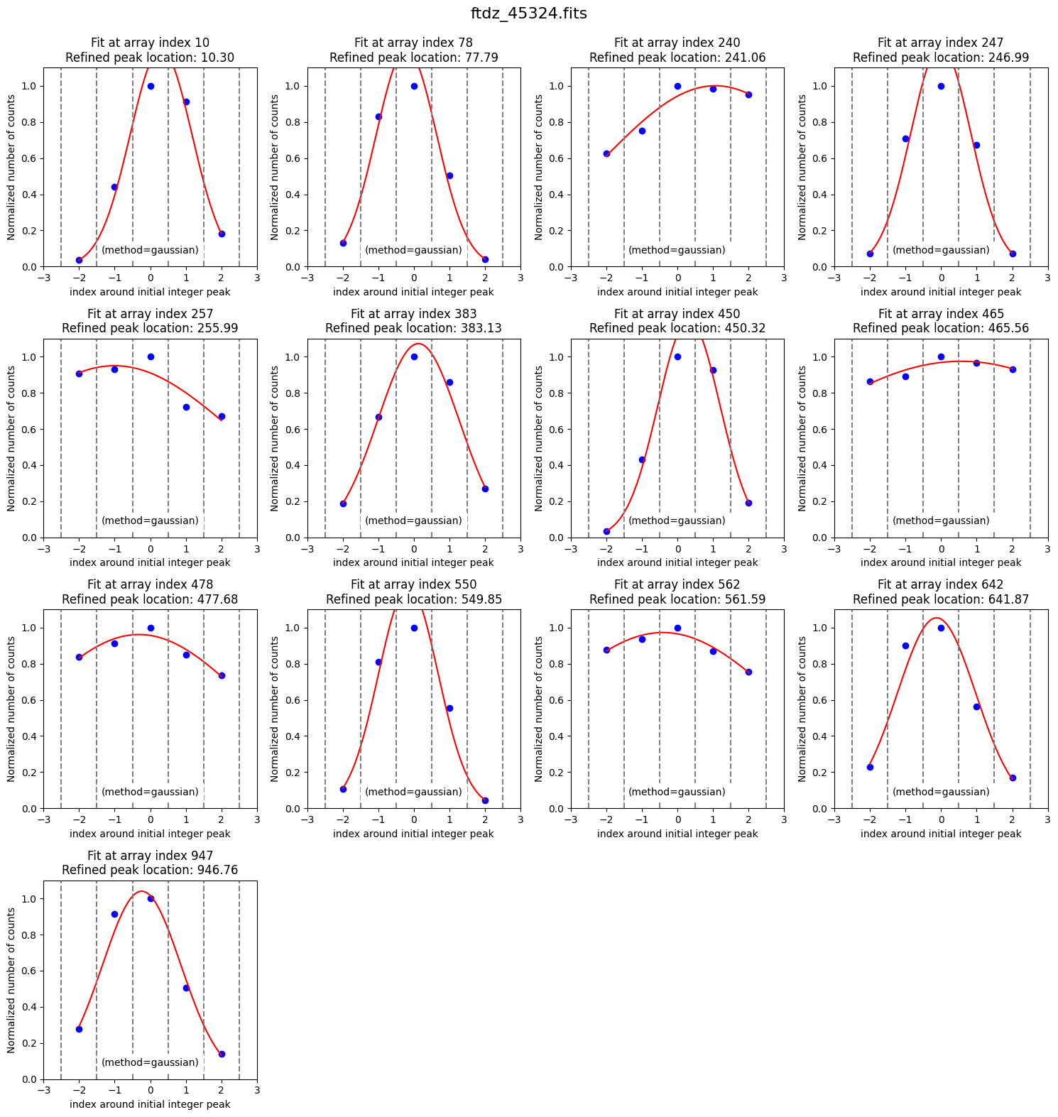
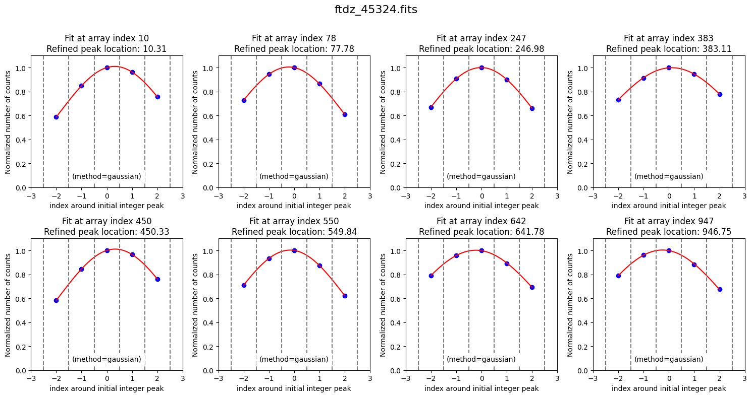
Some peaks found in the wings of bright lines are spurious. We can get rid of them by smoothing the spectrum (sigma_smooth=2; this parameter is updated in the wavecalib object and if we’re satisfied with it, there’s no need to specify it again).
xpeaks_reference, ixpeaks_reference, spectrum_reference = wavecalib.compute_xpeaks_reference(
    data=data,
    ns_range=ns_range,
    sigma_smooth=2,
    plot_spectrum=True,
    plot_peaks=True,
    title=input_filename
)
The latest values of the parameters we have modified have been stored.
wavecalib
TeaWaveCalibration(
    ns_window=11,
    threshold=50,
    sigma_smooth=2,
    nx_window=5,
    delta_flux=0,
    method='gaussian',
    degree_cdistortion=1,
    degree_wavecalib=1,
    peak_wavelengths=None,
    _nlines_reference=None,
    _naxis1=1024,
    _naxis2=250,
    _xpeaks_all_lines_array=None,
    _valid_scans=None,
    _list_poly_cdistortion=None,
    _array_poly_wav=None,
    _array_poly_pix=None,
    _array_residual_std_wav=None,
    _array_residual_std_pix=None,
    _array_crval1_linear=None,
    _array_cdelt1_linear=None,
    _array_crmax1_linear=None
)
The final positions of the lines (in array coordinates, starting from 0) are
xpeaks_reference
Note that these positions are not stored as an attribute in the wavecalib object we created, but rather we have them stored in an external array that we can modify as we wish. The advantage of this approach is that we can easily remove some of the peaks. For example, we can remove:
saturated lines
unreliable peaks from faint lines
peaks from lines whose wavelengths we do not know
In our case, there’s no need to remove any peaks because the 8 we found are useful. But suppose we wanted to remove the third and fifth peaks (indices 2 and 4). We can remove them from the array using NumPy functionality.
xpeaks_reference_new = np.delete(xpeaks_reference, [2, 4])
xpeaks_reference_new
The above has not modified the original array.
xpeaks_reference
Wavelength Calibration of the Reference Spectrum#
We need to specify the wavelengths of the peaks we consider useful and for which we know the wavelengths. For this, we use the method define_peak_wavelengths(), which requires the wavelengths (in increasing order) of the peaks, with units. This function needs two arguments: the array with the detected peaks and the array of wavelengths (the first parameter is only used to check that the number of elements is the same in both arrays).
wavelengths_reference= np.array(
    [
        6506.528, 6532.880, 6598.953,
        6652.090, 6678.200, 6717.043,
        6752.832, 6871.290
    ]
) * u.Angstrom

wavecalib.define_peak_wavelengths(
    xpeaks=xpeaks_reference,
    wavelengths= wavelengths_reference
)
The wavelengths entered are stored in the peak_wavelengths attribute.
wavecalib
TeaWaveCalibration(
    ns_window=11,
    threshold=50,
    sigma_smooth=2,
    nx_window=5,
    delta_flux=0,
    method='gaussian',
    degree_cdistortion=1,
    degree_wavecalib=1,
    peak_wavelengths=<Quantity [6506.528, 6532.88 , 6598.953, 6652.09 , 6678.2  , 6717.043,
           6752.832, 6871.29 ] Angstrom>,
    _nlines_reference=None,
    _naxis1=1024,
    _naxis2=250,
    _xpeaks_all_lines_array=None,
    _valid_scans=None,
    _list_poly_cdistortion=None,
    _array_poly_wav=None,
    _array_poly_pix=None,
    _array_residual_std_wav=None,
    _array_residual_std_pix=None,
    _array_crval1_linear=None,
    _array_cdelt1_linear=None,
    _array_crmax1_linear=None
)
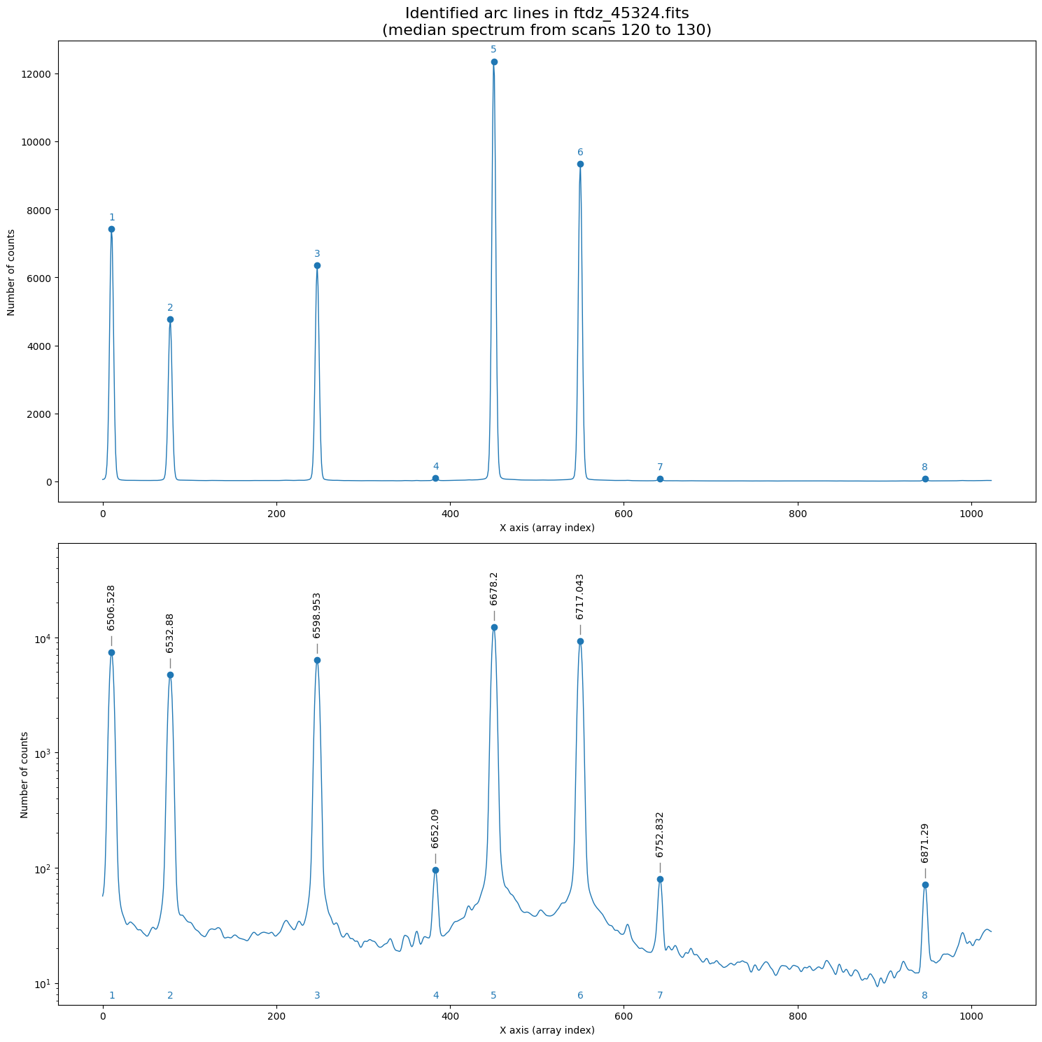
We can display the spectrum with the introduced wavelengths (we also save the plot in a PDF file).
wavecalib.overplot_identified_lines(
    xpeaks=xpeaks_reference,
    spectrum=spectrum_reference,
    title=f'Identified arc lines in {input_filename}\n'
          f'(median spectrum from scans {ns_range.fits.start} to {ns_range.fits.stop})',
    pdf_output=f'plot_{Path(input_filename).stem}_identified_lines.pdf'
)
--> Saving PDF file: plot_ftdz_45324_identified_lines.pdf
Now we can proceed with the calculation of the wavelength calibration polynomial. We do this using the fit_xpeaks_wavelengths() method, which requires the array with the peak positions as an argument. In this case, we also enable it to display additional information on screen (debug=True) and force it to graphically show the result (plots=True).
poly_fits_wav, residual_std_wav, poly_fits_pix, residual_std_pix, \
crval1_linear, cdelt1_linear, crmax1_linear = wavecalib.fit_xpeaks_wavelengths(
    xpeaks=xpeaks_reference,
    debug=True,
    plots=True,
    title=input_filename
)
>>> CRPIX1.............: 1.0 pix
>>> CRVAL1 linear scale: 6502.675086411521 Angstrom
>>> CDELT1 linear scale: 0.38961619272091447 Angstrom / pix
>>> CRMAX1 linear scale: 6901.252451565017 Angstrom

>>> Fitted coefficients pixel(wavelength):
 [-1.66889508e+04  2.56662844e+00]
>>> Residual std.........................: 0.4222488109410994 pix

>>> Fitted coefficients wavelength(pixel):
 [6.50228547e+03 3.89616193e-01]
>>> Residual std.........................: 0.16451497409980437 Angstrom
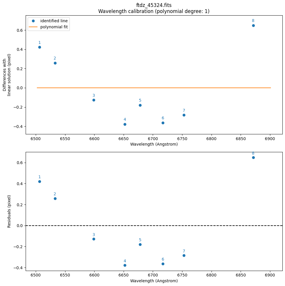
By default, it has used a polynomial of degree degree_wavecalib=1. We are going to increase it to a polynomial of degree 3. Since this fit will be valid, we also save the plots in a PDF file.
poly_fits_wav, residual_std_wav, poly_fits_pix, residual_std_pix, \
crval1_linear, cdelt1_linear, crmax1_linear = wavecalib.fit_xpeaks_wavelengths(
    xpeaks=xpeaks_reference,
    degree_wavecalib=3,
    debug=True,
    plots=True,
    title=input_filename,
    pdf_output=f'plot_{Path(input_filename).stem}_wavecalib.pdf'
)
>>> CRPIX1.............: 1.0 pix
>>> CRVAL1 linear scale: 6502.50004651459 Angstrom
>>> CDELT1 linear scale: 0.38938661758667953 Angstrom / pix
>>> CRMAX1 linear scale: 6900.8425563057635 Angstrom

>>> Fitted coefficients pixel(wavelength):
 [-2.54126929e+04  6.65567621e+00 -6.37642087e-04  3.30842991e-08]
>>> Residual std.........................: 0.09176281215626683 pix

>>> Fitted coefficients wavelength(pixel):
 [ 6.50210939e+03  3.90659576e-01 -4.74427072e-07 -7.49495201e-10]
>>> Residual std.........................: 0.03573121104577058 Angstrom
--> Saving PDF file: plot_ftdz_45324_wavecalib.pdf

The function first performs a fit to a polynomial of the form pixel(wavelength) (using wavelength as the independent variable and pixel as the dependent variable). We do it this way because we expect to have more uncertainty in the peak positions (determined by fitting the line profiles) than in the wavelengths of the lines (which are supposedly tabulated and known with high precision). This initial fit is then inverted to obtain a polynomial that provides wavelength(pixel), which is more convenient for predicting the wavelength of any pixel. The function has returned the following parameters:
poly_fits_wav: corresponds to the polynomialwavelength(pixel)residual_std_wav: residual standard deviation corresponding to the previous fit (in wavelength units)poly_fits_pix: corresponds to the polynomialpixel(wavelength)residual_std_pix: residual standard deviation corresponding to the previous fit (in pixels)crval1_linear: value of CRVAL1 (wavelength of the first pixel) in the linear fit approximationcdelt1_linear: value of CDELT1 (reciprocal linear dispersion; in this case in Angstrom/pixel)crmax1_linear: this parameter is not a standard FITS keyword, but it is useful. It indicates the wavelength at the center of the pixel corresponding to NAXIS1.
The last value of degree_wavecal has been stored in the wavecalib object, so it will be the value used (unless we decide to change it again).
wavecalib
TeaWaveCalibration(
    ns_window=11,
    threshold=50,
    sigma_smooth=2,
    nx_window=5,
    delta_flux=0,
    method='gaussian',
    degree_cdistortion=1,
    degree_wavecalib=3,
    peak_wavelengths=<Quantity [6506.528, 6532.88 , 6598.953, 6652.09 , 6678.2  , 6717.043,
           6752.832, 6871.29 ] Angstrom>,
    _nlines_reference=None,
    _naxis1=1024,
    _naxis2=250,
    _xpeaks_all_lines_array=None,
    _valid_scans=None,
    _list_poly_cdistortion=None,
    _array_poly_wav=None,
    _array_poly_pix=None,
    _array_residual_std_wav=None,
    _array_residual_std_pix=None,
    _array_crval1_linear=None,
    _array_cdelt1_linear=None,
    _array_crmax1_linear=None
)
Searching for the lines across the entire image#
If the C distortion of the image is not too severe, it is likely that we can fit the position of all selected peaks using an automatic procedure that only requires the initial position of the peaks.
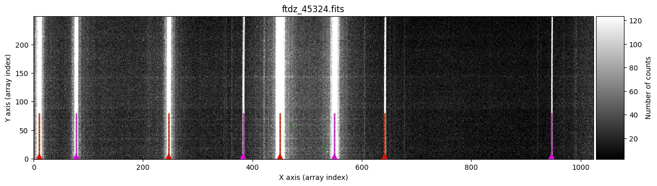
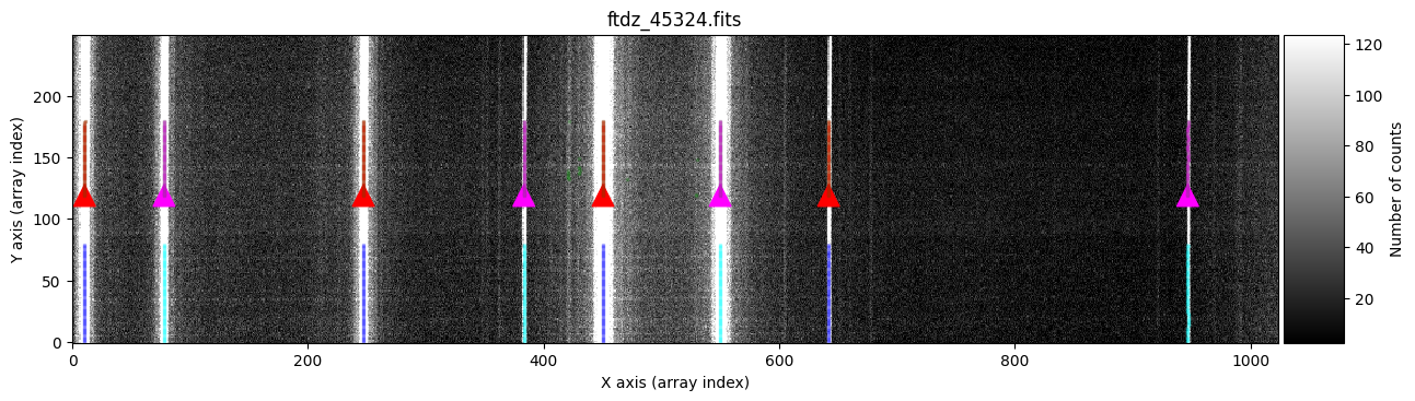
We run this procedure using the compute_xpeaks_image() method, to which we must pass the 2D image array data and the peak positions xpeaks_reference for which we know the associated wavelengths. This function can also graphically display all the peaks found for each spectrum and the association of those peaks to each particular line (plots=True). The parameter disable_tqdm=False indicates that we want to see a progress bar in the notebook as the calculations are performed.
wavecalib.compute_xpeaks_image(
    data=data,
    xpeaks_reference=xpeaks_reference,
    plots=True,
    disable_tqdm=False,
    title=input_filename
)
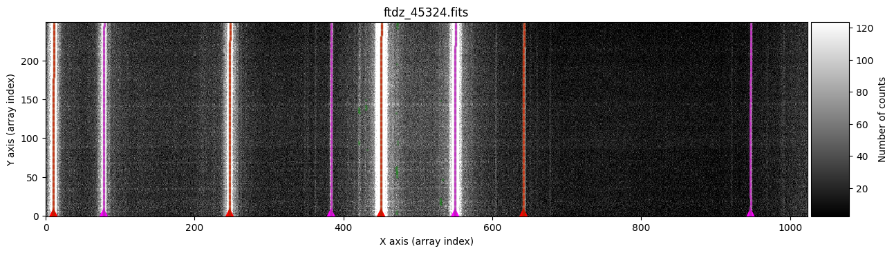
In green, we see peaks found in the different spectra. The function selects, for each line, the peak closest to the average (median) position of the peaks in the ns_window nearest spectra (in this case, we are using the default value ns_window=11). This ensures that the predicted position for the peaks in each new spectrum follows the C distortion calculated from neighboring spectra. Since we haven’t specified a particular spectral region, the procedure starts with the first spectrum (at the bottom) and progresses up to the spectrum corresponding to NAXIS2 (this is also graphically indicated by the colored triangles shown over the starting spectrum). It is therefore advisable that the peaks in the first spectra are relatively close to the position indicated in xpeaks_reference. The peaks of each line are marked in red (odd lines) and purple (even lines). For cases where the C distortion is significant, it is possible to use a more elaborate method that allows fitting different intervals along the spectral direction (see example below).
In the example we are considering, the automatic method works perfectly.
Fitting the C distortion#
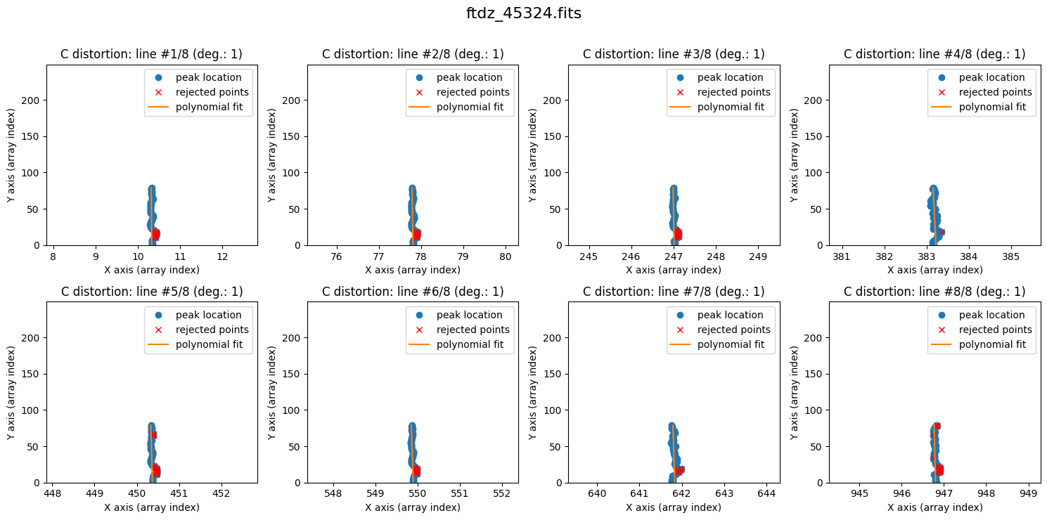
We can now proceed with fitting the C distortion for each line. By default, a polynomial of degree 1 is used.
wavecalib.fit_cdistortion(
    plots=True,
    title=input_filename
)
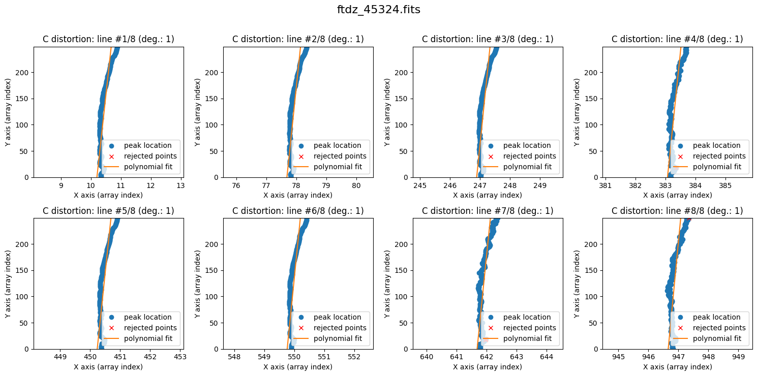
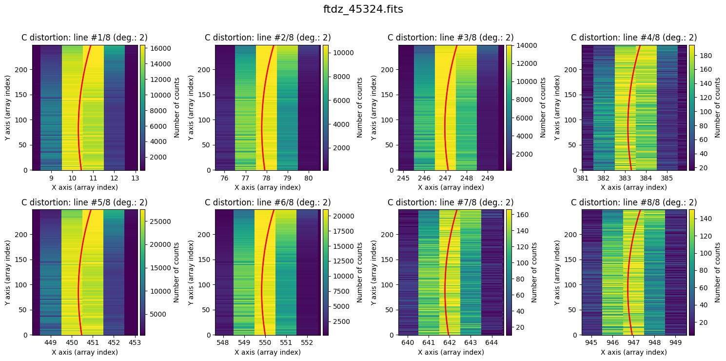
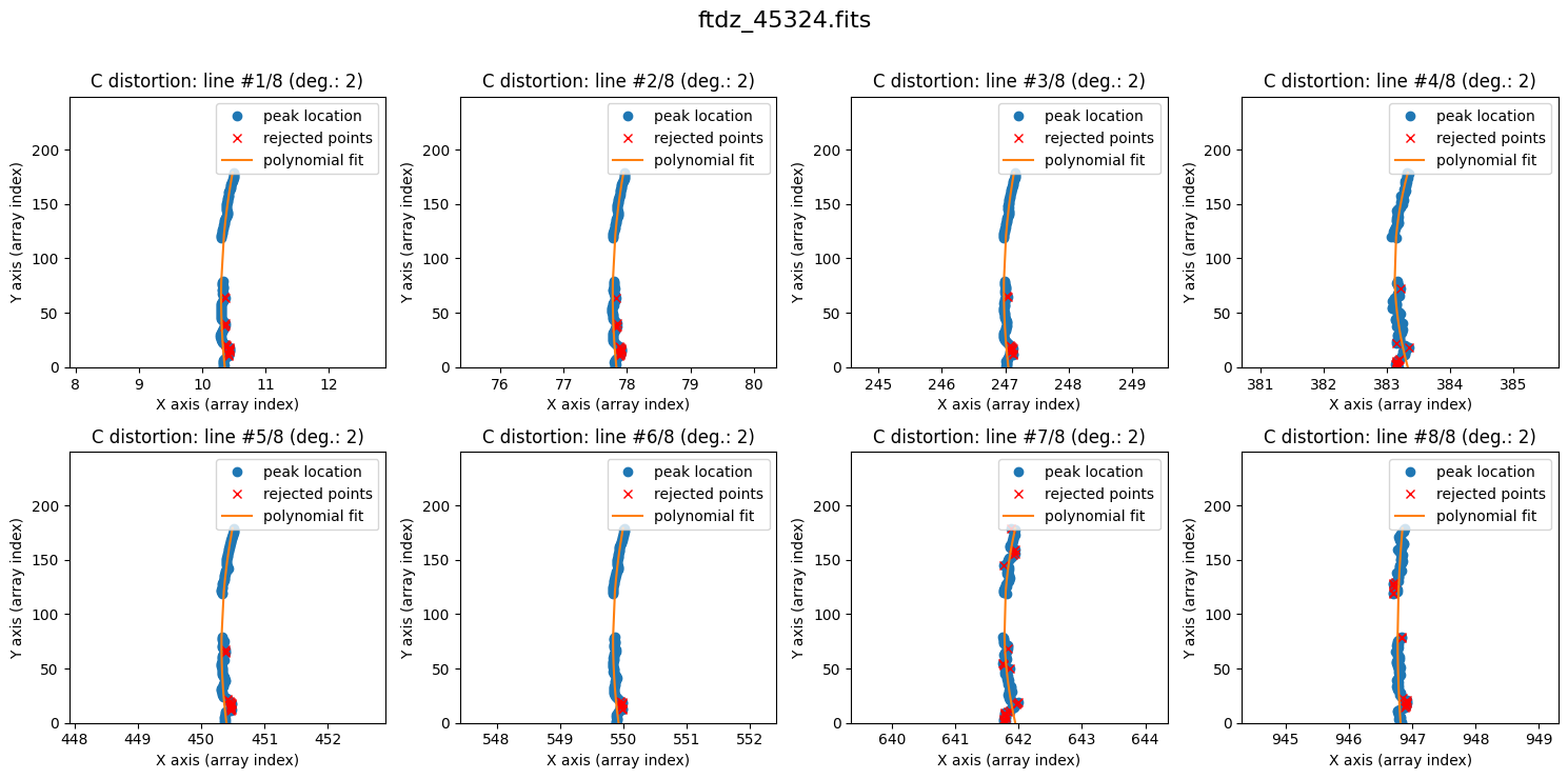
The lines show curvature, and a polynomial of degree 1 is not sufficient. We increase the degree of the polynomial to fit the C distortion using degree_cdistortion=2.
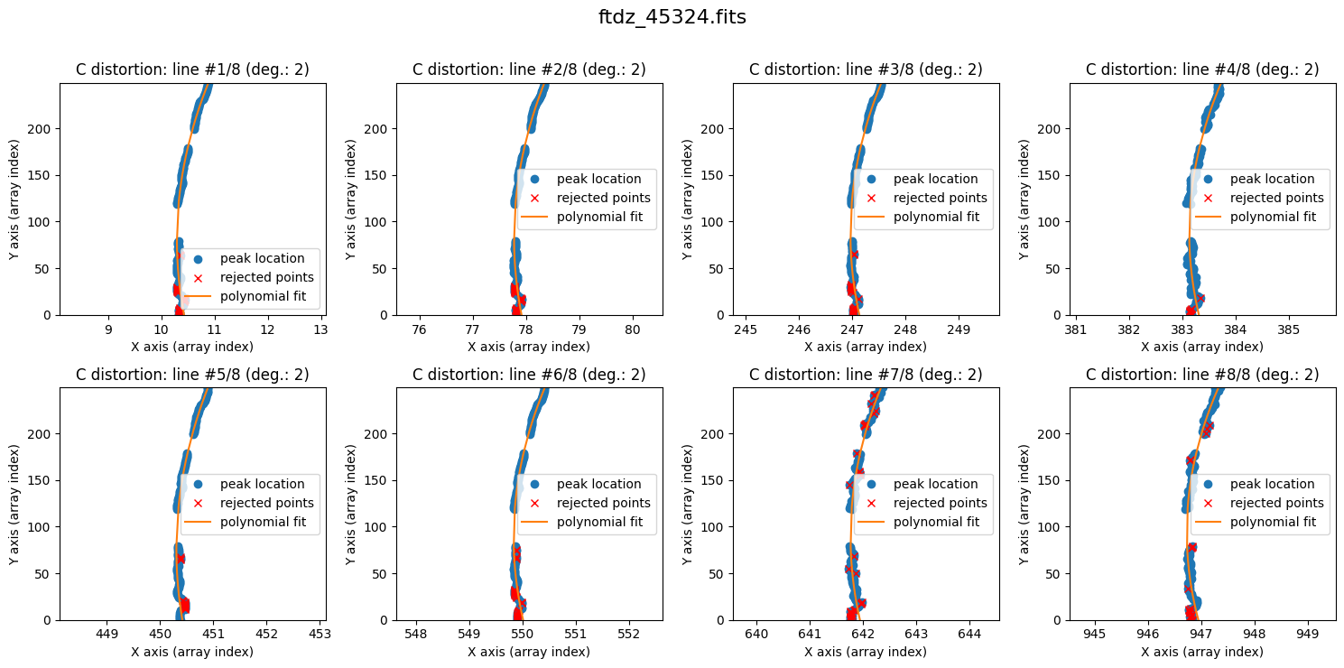
wavecalib.fit_cdistortion(
    degree_cdistortion=2,
    plots=True,
    title=input_filename
)
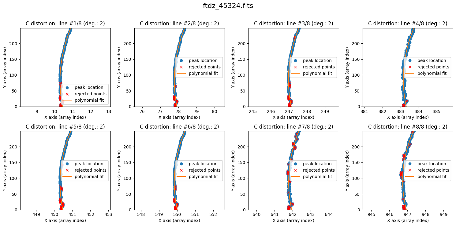
The result is now clearly better. The fit is performed iteratively by removing points that deviate more than 3 times the standard deviation (the outliers are shown in red). The last value of degree_cdistortion is stored as an attribute of the wavecalib object, so we don’t need to specify it again explicitly. New attributes have been updated in this object to store the selected peaks in each spectrum, as well as the polynomials fitted to the C distortion of each line.
wavecalib
TeaWaveCalibration(
    ns_window=11,
    threshold=50,
    sigma_smooth=2,
    nx_window=5,
    delta_flux=0,
    method='gaussian',
    degree_cdistortion=2,
    degree_wavecalib=3,
    peak_wavelengths=<Quantity [6506.528, 6532.88 , 6598.953, 6652.09 , 6678.2  , 6717.043,
           6752.832, 6871.29 ] Angstrom>,
    _nlines_reference=8,
    _naxis1=1024,
    _naxis2=250,
    _xpeaks_all_lines_array=array([[ 10.32905234,  77.80555129, 247.02193551, ..., 549.89121403,
        641.77328117, 946.83276802],
       [ 10.33260378,  77.81100587, 247.01588494, ..., 549.89207883,
        641.76059442, 946.82642287],
       [ 10.34568947,  77.81000046, 247.02368721, ..., 549.88797079,
        641.79459232, 946.80807042],
       ...,
       [ 10.87332486,  78.33716115, 247.54521942, ..., 550.4003933 ,
        642.31360776, 947.30193393],
       [ 10.87840224,  78.34162022, 247.54803766, ..., 550.40171927,
        642.33887363, 947.261077  ],
       [ 10.88042931,  78.34612774, 247.55216   , ..., 550.40582838,
        642.36933702, 947.36151689]], shape=(250, 8)),
    _valid_scans=array([ True,  True,  True,  True,  True,  True,  True,  True,  True,
        True,  True,  True,  True,  True,  True,  True,  True,  True,
        True,  True,  True,  True,  True,  True,  True,  True,  True,
        True,  True,  True,  True,  True,  True,  True,  True,  True,
        True,  True,  True,  True,  True,  True,  True,  True,  True,
        True,  True,  True,  True,  True,  True,  True,  True,  True,
        True,  True,  True,  True,  True,  True,  True,  True,  True,
        True,  True,  True,  True,  True,  True,  True,  True,  True,
        True,  True,  True,  True,  True,  True,  True,  True,  True,
        True,  True,  True,  True,  True,  True,  True,  True,  True,
        True,  True,  True,  True,  True,  True,  True,  True,  True,
        True,  True,  True,  True,  True,  True,  True,  True,  True,
        True,  True,  True,  True,  True,  True,  True,  True,  True,
        True,  True,  True,  True,  True,  True,  True,  True,  True,
        True,  True,  True,  True,  True,  True,  True,  True,  True,
        True,  True,  True,  True,  True,  True,  True,  True,  True,
        True,  True,  True,  True,  True,  True,  True,  True,  True,
        True,  True,  True,  True,  True,  True,  True,  True,  True,
        True,  True,  True,  True,  True,  True,  True,  True,  True,
        True,  True,  True,  True,  True,  True,  True,  True,  True,
        True,  True,  True,  True,  True,  True,  True,  True,  True,
        True,  True,  True,  True,  True,  True,  True,  True,  True,
        True,  True,  True,  True,  True,  True,  True,  True,  True,
        True,  True,  True,  True,  True,  True,  True,  True,  True,
        True,  True,  True,  True,  True,  True,  True,  True,  True,
        True,  True,  True,  True,  True,  True,  True,  True,  True,
        True,  True,  True,  True,  True,  True,  True,  True,  True,
        True,  True,  True,  True,  True,  True,  True]),
    _list_poly_cdistortion=[Polynomial([ 1.04334756e+01, -3.43444345e-03,  2.11570051e-05], domain=[-1.,  1.], window=[-1.,  1.], symbol='x'), Polynomial([ 7.79139467e+01, -3.44029154e-03,  2.07424667e-05], domain=[-1.,  1.], window=[-1.,  1.], symbol='x'), Polynomial([ 2.47129311e+02, -3.69188047e-03,  2.16317679e-05], domain=[-1.,  1.], window=[-1.,  1.], symbol='x'), Polynomial([ 3.83306360e+02, -3.82106978e-03,  2.21481209e-05], domain=[-1.,  1.], window=[-1.,  1.], symbol='x'), Polynomial([ 4.50475429e+02, -3.71155824e-03,  2.19920696e-05], domain=[-1.,  1.], window=[-1.,  1.], symbol='x'), Polynomial([ 5.49998907e+02, -3.85060381e-03,  2.21252317e-05], domain=[-1.,  1.], window=[-1.,  1.], symbol='x'), Polynomial([ 6.41946418e+02, -3.85681639e-03,  2.18820614e-05], domain=[-1.,  1.], window=[-1.,  1.], symbol='x'), Polynomial([ 9.46940466e+02, -4.50828822e-03,  2.43954520e-05], domain=[-1.,  1.], window=[-1.,  1.], symbol='x')],
    _array_poly_wav=None,
    _array_poly_pix=None,
    _array_residual_std_wav=None,
    _array_residual_std_pix=None,
    _array_crval1_linear=None,
    _array_cdelt1_linear=None,
    _array_crmax1_linear=None
)
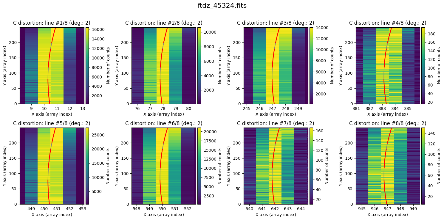
Finally, it is also useful to display the calculated C distortion over the original image, zooming in on each line.
wavecalib.plot_cdistortion(data, title=input_filename)
Partial fits#
In particular cases where we need to ignore some spectra during the fitting, we can use a more refined procedure, which can also help us use sky lines (instead of arc lines) to perform the wavelength calibration (in this case, it may be essential to skip object spectra that interfere with the peak detection process).
Since we are continuing with the same example image, we delete the previously fitted C distortion polynomials but preserve the parameters we have identified as suitable for this image (ns_window, threshold, sigma_smooth, nx_window, method, degree_cdistortion, degree_wavecal, peak_wavelengths).
We achieve this using the reset_image() method.
wavecalib.reset_image()
wavecalib
TeaWaveCalibration(
    ns_window=11,
    threshold=50,
    sigma_smooth=2,
    nx_window=5,
    delta_flux=0,
    method='gaussian',
    degree_cdistortion=2,
    degree_wavecalib=3,
    peak_wavelengths=<Quantity [6506.528, 6532.88 , 6598.953, 6652.09 , 6678.2  , 6717.043,
           6752.832, 6871.29 ] Angstrom>,
    _nlines_reference=None,
    _naxis1=None,
    _naxis2=None,
    _xpeaks_all_lines_array=None,
    _valid_scans=None,
    _list_poly_cdistortion=None,
    _array_poly_wav=None,
    _array_poly_pix=None,
    _array_residual_std_wav=None,
    _array_residual_std_pix=None,
    _array_crval1_linear=None,
    _array_cdelt1_linear=None,
    _array_crmax1_linear=None
)
As the C distortion in this image is not very large, the peak positions stored in xpeaks_reference are a good starting point for peak searching in any spectrum of the image.
We now proceed to calculate the C distortion, skipping the spectra in the intervals [81, 119] and [181, 199]. In other words, we fit the spectra corresponding to the intervals [1, 80], [120, 180], and [200, 250] (the numbers follow the FITS convention, which starts at 1; however, the plots show the array index, which starts at 0).
We begin by fitting the interval [1, 80].
ns_range1 = tea.SliceRegion1D(np.s_[1:80], mode='fits')

wavecalib.compute_xpeaks_image(
    data=data,
    xpeaks_reference=xpeaks_reference,
    ns_range=ns_range1,
    plots=True,
    title=input_filename,
    disable_tqdm=False
)
The peaks of each line are marked in red (odd lines) and purple (even lines).
We continue with the interval [120, 180]. In this case, we will perform the peak search from top to bottom (that is, starting from spectrum 180 and going down to 120). This option (which in this example is not relevant) can be useful when we have images with strong C distortion and when the xpeaks_reference positions have been calculated for an average spectrum from the top part of the image. To indicate that we want to move from top to bottom in the peak search, we use the parameter direction='down'; this parameter, by default, is 'up'.
ns_range2 = tea.SliceRegion1D(np.s_[120:180], mode='fits')

wavecalib.compute_xpeaks_image(
    data=data,
    xpeaks_reference=xpeaks_reference,
    ns_range=ns_range2,
    direction='down',
    plots=True,
    title=input_filename,
    disable_tqdm=False
)
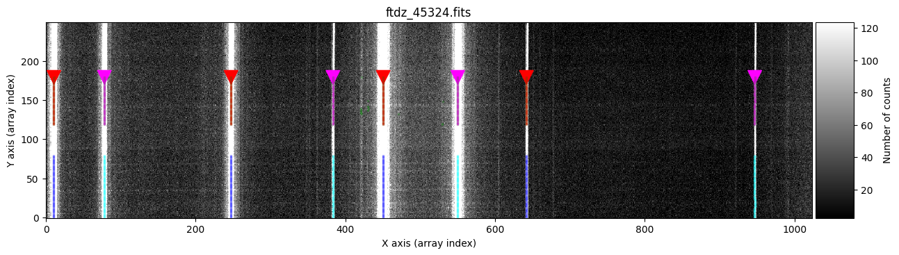
The new peaks of each line are marked in red (odd lines) and purple (even lines), while the previously calculated peaks appear in blue (odd lines) and cyan (even lines). Note that it is graphically indicated that the peak search has been performed from top to bottom.
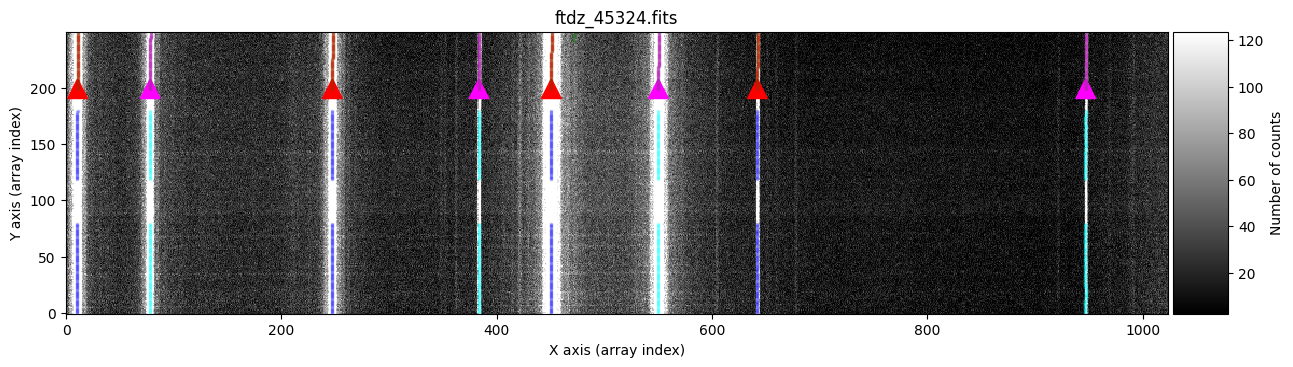
We add the peaks in a third interval [200, 250].
ns_range3 = tea.SliceRegion1D(np.s_[200:250], mode='fits')

wavecalib.compute_xpeaks_image(
    data=data,
    xpeaks_reference=xpeaks_reference,
    ns_range=ns_range3,
    plots=True,
    title=input_filename,
    disable_tqdm=False
)
wavecalib.fit_cdistortion(plots=True, title=input_filename)
We can display the calculated C distortion over the original image by zooming in on each line.
wavecalib.plot_cdistortion(data, title=input_filename)
wavecalib
TeaWaveCalibration(
    ns_window=11,
    threshold=50,
    sigma_smooth=2,
    nx_window=5,
    delta_flux=0,
    method='gaussian',
    degree_cdistortion=2,
    degree_wavecalib=3,
    peak_wavelengths=<Quantity [6506.528, 6532.88 , 6598.953, 6652.09 , 6678.2  , 6717.043,
           6752.832, 6871.29 ] Angstrom>,
    _nlines_reference=8,
    _naxis1=1024,
    _naxis2=250,
    _xpeaks_all_lines_array=array([[ 10.32905234,  77.80555129, 247.02193551, ..., 549.89121403,
        641.77328117, 946.83276802],
       [ 10.33260378,  77.81100587, 247.01588494, ..., 549.89207883,
        641.76059442, 946.82642287],
       [ 10.34568947,  77.81000046, 247.02368721, ..., 549.88797079,
        641.79459232, 946.80807042],
       ...,
       [ 10.87332486,  78.33716115, 247.54521942, ..., 550.4003933 ,
        642.31360776, 947.30193393],
       [ 10.87840224,  78.34162022, 247.54803766, ..., 550.40171927,
        642.33887363, 947.261077  ],
       [ 10.88042931,  78.34612774, 247.55216   , ..., 550.40582838,
        642.36933702, 947.36151689]], shape=(250, 8)),
    _valid_scans=array([ True,  True,  True,  True,  True,  True,  True,  True,  True,
        True,  True,  True,  True,  True,  True,  True,  True,  True,
        True,  True,  True,  True,  True,  True,  True,  True,  True,
        True,  True,  True,  True,  True,  True,  True,  True,  True,
        True,  True,  True,  True,  True,  True,  True,  True,  True,
        True,  True,  True,  True,  True,  True,  True,  True,  True,
        True,  True,  True,  True,  True,  True,  True,  True,  True,
        True,  True,  True,  True,  True,  True,  True,  True,  True,
        True,  True,  True,  True,  True,  True,  True,  True, False,
       False, False, False, False, False, False, False, False, False,
       False, False, False, False, False, False, False, False, False,
       False, False, False, False, False, False, False, False, False,
       False, False, False, False, False, False, False, False, False,
       False, False,  True,  True,  True,  True,  True,  True,  True,
        True,  True,  True,  True,  True,  True,  True,  True,  True,
        True,  True,  True,  True,  True,  True,  True,  True,  True,
        True,  True,  True,  True,  True,  True,  True,  True,  True,
        True,  True,  True,  True,  True,  True,  True,  True,  True,
        True,  True,  True,  True,  True,  True,  True,  True,  True,
        True,  True,  True,  True,  True,  True,  True,  True,  True,
       False, False, False, False, False, False, False, False, False,
       False, False, False, False, False, False, False, False, False,
       False,  True,  True,  True,  True,  True,  True,  True,  True,
        True,  True,  True,  True,  True,  True,  True,  True,  True,
        True,  True,  True,  True,  True,  True,  True,  True,  True,
        True,  True,  True,  True,  True,  True,  True,  True,  True,
        True,  True,  True,  True,  True,  True,  True,  True,  True,
        True,  True,  True,  True,  True,  True,  True]),
    _list_poly_cdistortion=[Polynomial([ 1.04290791e+01, -3.35373804e-03,  2.08528342e-05], domain=[-1.,  1.], window=[-1.,  1.], symbol='x'), Polynomial([ 7.79112922e+01, -3.41127839e-03,  2.06453080e-05], domain=[-1.,  1.], window=[-1.,  1.], symbol='x'), Polynomial([ 2.47137885e+02, -3.84749428e-03,  2.21246396e-05], domain=[-1.,  1.], window=[-1.,  1.], symbol='x'), Polynomial([ 3.83311403e+02, -4.11520871e-03,  2.32906296e-05], domain=[-1.,  1.], window=[-1.,  1.], symbol='x'), Polynomial([ 4.50423650e+02, -2.97686243e-03,  1.96822658e-05], domain=[-1.,  1.], window=[-1.,  1.], symbol='x'), Polynomial([ 5.50006348e+02, -4.01762966e-03,  2.27052407e-05], domain=[-1.,  1.], window=[-1.,  1.], symbol='x'), Polynomial([ 6.41948193e+02, -3.96551351e-03,  2.22975616e-05], domain=[-1.,  1.], window=[-1.,  1.], symbol='x'), Polynomial([ 9.46946237e+02, -4.63707812e-03,  2.46937643e-05], domain=[-1.,  1.], window=[-1.,  1.], symbol='x')],
    _array_poly_wav=None,
    _array_poly_pix=None,
    _array_residual_std_wav=None,
    _array_residual_std_pix=None,
    _array_crval1_linear=None,
    _array_cdelt1_linear=None,
    _array_crmax1_linear=None
)
In the previous steps, we could also have used partial fits of the C distortion (using a low-degree polynomial) to predict the expected position of the lines. This should allow us to correct images with pronounced C distortion, for which using a single xpeaks_reference array may not be a good idea.
wavecalib.reset_image()
wavecalib
TeaWaveCalibration(
    ns_window=11,
    threshold=50,
    sigma_smooth=2,
    nx_window=5,
    delta_flux=0,
    method='gaussian',
    degree_cdistortion=2,
    degree_wavecalib=3,
    peak_wavelengths=<Quantity [6506.528, 6532.88 , 6598.953, 6652.09 , 6678.2  , 6717.043,
           6752.832, 6871.29 ] Angstrom>,
    _nlines_reference=None,
    _naxis1=None,
    _naxis2=None,
    _xpeaks_all_lines_array=None,
    _valid_scans=None,
    _list_poly_cdistortion=None,
    _array_poly_wav=None,
    _array_poly_pix=None,
    _array_residual_std_wav=None,
    _array_residual_std_pix=None,
    _array_crval1_linear=None,
    _array_cdelt1_linear=None,
    _array_crmax1_linear=None
)
We start the procedure by fitting the spectra in the interval [1, 80].
print(ns_range1)
SliceRegion1D(slice(1, 80, None), mode="fits")
wavecalib.compute_xpeaks_image(
    data=data,
    xpeaks_reference=xpeaks_reference,
    ns_range=ns_range1,
    plots=True,
    title=input_filename,
    disable_tqdm=False
)
We calculate the C distortion. In this case, extrapolating with a degree-2 polynomial (which introduces curvature) can be risky, and a more conservative option is to start with a degree-1 polynomial.
wavecalib.fit_cdistortion(degree_cdistortion=1, plots=True, title=input_filename)
Using the predict_cdistortion() method, we can extrapolate the position of the lines for any spectrum, using the polynomials calculated so far to model the C distortion.
We can predict, for example, the expected position of the peaks for spectrum number 120 (following the FITS convention).
xpeaks_reference = wavecalib.predict_cdistortion(ns_fits=120)
xpeaks_reference
The new xpeaks_reference values will be a good estimate of the expected peak positions in spectrum number 120.
print(ns_range2)
SliceRegion1D(slice(120, 180, None), mode="fits")
wavecalib.compute_xpeaks_image(
    data=data,
    xpeaks_reference=xpeaks_reference,
    ns_range=ns_range2,
    plots=True,
    title=input_filename,
    disable_tqdm=False
)
We can now increase the degree of the polynomial to fit the C distortion.
wavecalib.fit_cdistortion(degree_cdistortion=2, plots=True, title=input_filename)
We once again predict the peak positions, this time for spectrum number 200.
xpeaks_reference = wavecalib.predict_cdistortion(ns_fits=200)
xpeaks_reference
We now search for the peaks in the last spatial interval.
print(ns_range3)
SliceRegion1D(slice(200, 250, None), mode="fits")
wavecalib.compute_xpeaks_image(
    data=data,
    xpeaks_reference=xpeaks_reference,
    ns_range=ns_range3,
    plots=True,
    title=input_filename,
    disable_tqdm=False
)
We finish with the calculation of distortion C.
wavecalib.fit_cdistortion(plots=True, title=input_filename)
wavecalib
TeaWaveCalibration(
    ns_window=11,
    threshold=50,
    sigma_smooth=2,
    nx_window=5,
    delta_flux=0,
    method='gaussian',
    degree_cdistortion=2,
    degree_wavecalib=3,
    peak_wavelengths=<Quantity [6506.528, 6532.88 , 6598.953, 6652.09 , 6678.2  , 6717.043,
           6752.832, 6871.29 ] Angstrom>,
    _nlines_reference=8,
    _naxis1=1024,
    _naxis2=250,
    _xpeaks_all_lines_array=array([[ 10.32905234,  77.80555129, 247.02193551, ..., 549.89121403,
        641.77328117, 946.83276802],
       [ 10.33260378,  77.81100587, 247.01588494, ..., 549.89207883,
        641.76059442, 946.82642287],
       [ 10.34568947,  77.81000046, 247.02368721, ..., 549.88797079,
        641.79459232, 946.80807042],
       ...,
       [ 10.87332486,  78.33716115, 247.54521942, ..., 550.4003933 ,
        642.31360776, 947.30193393],
       [ 10.87840224,  78.34162022, 247.54803766, ..., 550.40171927,
        642.33887363, 947.261077  ],
       [ 10.88042931,  78.34612774, 247.55216   , ..., 550.40582838,
        642.36933702, 947.36151689]], shape=(250, 8)),
    _valid_scans=array([ True,  True,  True,  True,  True,  True,  True,  True,  True,
        True,  True,  True,  True,  True,  True,  True,  True,  True,
        True,  True,  True,  True,  True,  True,  True,  True,  True,
        True,  True,  True,  True,  True,  True,  True,  True,  True,
        True,  True,  True,  True,  True,  True,  True,  True,  True,
        True,  True,  True,  True,  True,  True,  True,  True,  True,
        True,  True,  True,  True,  True,  True,  True,  True,  True,
        True,  True,  True,  True,  True,  True,  True,  True,  True,
        True,  True,  True,  True,  True,  True,  True,  True, False,
       False, False, False, False, False, False, False, False, False,
       False, False, False, False, False, False, False, False, False,
       False, False, False, False, False, False, False, False, False,
       False, False, False, False, False, False, False, False, False,
       False, False,  True,  True,  True,  True,  True,  True,  True,
        True,  True,  True,  True,  True,  True,  True,  True,  True,
        True,  True,  True,  True,  True,  True,  True,  True,  True,
        True,  True,  True,  True,  True,  True,  True,  True,  True,
        True,  True,  True,  True,  True,  True,  True,  True,  True,
        True,  True,  True,  True,  True,  True,  True,  True,  True,
        True,  True,  True,  True,  True,  True,  True,  True,  True,
       False, False, False, False, False, False, False, False, False,
       False, False, False, False, False, False, False, False, False,
       False,  True,  True,  True,  True,  True,  True,  True,  True,
        True,  True,  True,  True,  True,  True,  True,  True,  True,
        True,  True,  True,  True,  True,  True,  True,  True,  True,
        True,  True,  True,  True,  True,  True,  True,  True,  True,
        True,  True,  True,  True,  True,  True,  True,  True,  True,
        True,  True,  True,  True,  True,  True,  True]),
    _list_poly_cdistortion=[Polynomial([ 1.04290791e+01, -3.35373804e-03,  2.08528342e-05], domain=[-1.,  1.], window=[-1.,  1.], symbol='x'), Polynomial([ 7.79112922e+01, -3.41127839e-03,  2.06453080e-05], domain=[-1.,  1.], window=[-1.,  1.], symbol='x'), Polynomial([ 2.47137885e+02, -3.84749428e-03,  2.21246396e-05], domain=[-1.,  1.], window=[-1.,  1.], symbol='x'), Polynomial([ 3.83311403e+02, -4.11520871e-03,  2.32906296e-05], domain=[-1.,  1.], window=[-1.,  1.], symbol='x'), Polynomial([ 4.50423650e+02, -2.97686243e-03,  1.96822658e-05], domain=[-1.,  1.], window=[-1.,  1.], symbol='x'), Polynomial([ 5.50006348e+02, -4.01762966e-03,  2.27052407e-05], domain=[-1.,  1.], window=[-1.,  1.], symbol='x'), Polynomial([ 6.41948193e+02, -3.96551351e-03,  2.22975616e-05], domain=[-1.,  1.], window=[-1.,  1.], symbol='x'), Polynomial([ 9.46946237e+02, -4.63707812e-03,  2.46937643e-05], domain=[-1.,  1.], window=[-1.,  1.], symbol='x')],
    _array_poly_wav=None,
    _array_poly_pix=None,
    _array_residual_std_wav=None,
    _array_residual_std_pix=None,
    _array_crval1_linear=None,
    _array_cdelt1_linear=None,
    _array_crmax1_linear=None
)
Wavelength Calibration Calculation for the Entire Image#
Once a good modeling of the C distortion has been obtained for a specific number of lines, the only remaining step is to evaluate, for each spectrum, the expected position of the lines. The wavelengths of these lines are then fitted based on the position of the peaks, for all spectra in the image. This then provides a wavelength calibration polynomial for each spectrum.
This task is performed automatically using the fit_wavelengths() method.
The calibration polynomials are stored in an auxiliary FITS file with the following format:
Primary HDU: an image is saved in which each row contains the coefficients of the
wavelength(pixel)polynomial. That is,NAXIS1is equal to the degree of the wavelength calibration polynomial plus one (degree_wavecalib+1), whileNAXIS2remains the number of spectra in the original FITS image.Second HDU (extension number 1,
INV_POLY): contains the coefficients of thepixel(wavelength)polynomial, which is the one actually fitted when calculating the wavelength calibration.Third HDU (extension number 2,
CDISTOR): contains the coefficients of the polynomials fitted to each spectral line (C distortion).Fourth HDU (extension number 3,
COEFF): contains a binary table with five columns:residual_std_wav: residual standard deviation of the fit to thewavelength(pixel)polynomial.residual_std_pix: residual standard deviation of the fit to thepixel(wavelength)polynomial.crval1_linear: value of the FITS keywordCRVAL1, which stores the wavelength at the center of the first pixel (here we always assume the reference pixel isCRPIX1=1), in the linear approximation.cdelt1_linear: value of the FITS keywordCDELT1, which stores the reciprocal linear dispersion, evaluated in the linear approximation.crmax1_linear: value of the wavelength at the center of pixel numberNAXIS1, calculated assuming the linear approximation.
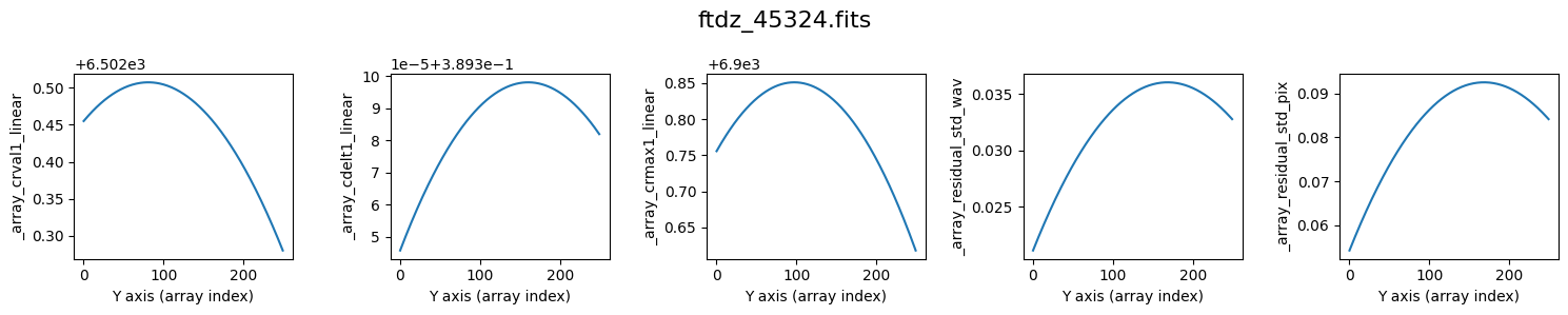
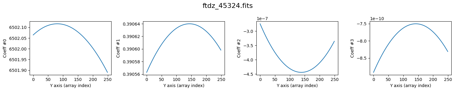
We perform the wavelength calibration. During the process, auxiliary plots are shown (plots=True) with the values of crval1_linear, cdelt1_linear, crmax1_linear, and residual_std, as well as the various coefficients of the wavelength calibration polynomial, as a function of the spectrum number.
# define additional information for the image header
history_list = [
    'Wavelength calibration',
    f'Input file: {input_filename}'
]

# name of the auxiliary FITS file
wavecal_filename = f'wavecal_{input_filename}'

# compute wavelength calibration and save result in auxiliary FITS file
wavecalib.fit_wavelengths(
    output_filename=wavecal_filename,
    history_list=history_list,
    plots=True,
    title=input_filename
)
>>> minimum CRVAL1 linear: 6502.280327548579 Angstrom
>>> maximum CRMAX1 linear: 6900.851045180415 Angstrom
>>> mean CDELT1..........: 0.38960969465477574 Angstrom
--> Saving result in FITS file: wavecal_ftdz_45324.fits
Reading the Calibration from the Auxiliary FITS File#
We can verify that the calibration we generated has been correctly stored in the auxiliary FITS file. To do this, we will create a new instance wavecalib_bis of the TeaWaveCalibration class, initializing it directly with the information stored in that file. Further below, we will check that the wavelength calibration it provides is the same as the one obtained from the initial wavecalib object.
wavecalib_bis = tea.TeaWaveCalibration.read(wavecal_filename)
>>> Reading file.........: wavecal_ftdz_45324.fits
>>> minimum CRVAL1 linear: 6502.280327548579 Angstrom
>>> maximum CRMAX1 linear: 6900.851045180415 Angstrom
>>> mean CDELT1..........: 0.38960969465477574 Angstrom
Applying the Wavelength Calibration#
Once all the wavelength calibration polynomials have been calculated, they just need to be applied to the images to be corrected. We can immediately apply the correction to the arc image.
Note that this procedure simultaneously corrects for C distortion and performs resampling on a linear wavelength scale. This method therefore does not require resampling the data twice: that is, it is not necessary to first correct for C distortion (which involves resampling) and then apply the wavelength calibration (which would again involve resampling the signal). By performing both tasks at once, we avoid correlating the errors twice.
Wavelength calibration requires providing two fundamental parameters:
CRVAL1: wavelength at the center of the first pixel (we are assumingCRPIX1=1).CDELT1: reciprocal linear dispersion, constant throughout the resulting spectrum.
crval1 = 6502 * u.Angstrom
cdelt1 = 0.390 * u.Angstrom / u.pixel
We are going to run the procedure twice: this way we can verify that the result is the same whether we use the wavecalib object or wavecalib_bis.
data_wavecalib = wavecalib.apply(
    data=data,
    crval1=crval1,
    cdelt1=cdelt1,
    disable_tqdm=False
)

data_wavecalib_bis = wavecalib_bis.apply(
    data=data,
    crval1=crval1,
    cdelt1=cdelt1,
    disable_tqdm=False
)
>>> Using CDELT1: 1 pix
>>> Using CRVAL1: 6502.0 Angstrom
>>> Using CDELT1: 0.39 Angstrom / pix
>>> Using CDELT1: 1 pix
>>> Using CRVAL1: 6502.0 Angstrom
>>> Using CDELT1: 0.39 Angstrom / pix
# difference between both calibrated arrays
diff = data_wavecalib - data_wavecalib_bis
print(diff.min(), diff.max())
0.0 0.0
We save the calibrated image to a FITS file. It is important not to forget to include in the FITS header the keywords that indicate the image is wavelength-calibrated. In this case, we take the header of the image (before being wavelength-calibrated) and complement it with the keywords CRPIX1, CRVAL1, CDELT1, CUNIT1, and CTYPE1.
header = fits.getheader(input_filename)
header['CRPIX1'] = (1, f'{u.pixel}')
header['CRVAL1'] = (crval1.value, f'{crval1.unit}')
header['CDELT1'] = (cdelt1.value, f'{cdelt1.unit}' )
header['CUNIT1'] = (f'{crval1.unit}', 'wavelength unit')
header['CTYPE1'] = ('AWAV', 'air wavelength')

hdu = fits.PrimaryHDU(header=header, data=data_wavecalib)
hdul = fits.HDUList([hdu])
hdul.writeto('dummy.fits', overwrite=True)
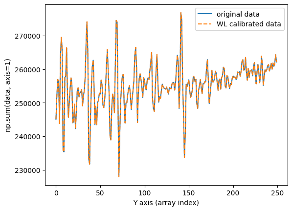
We verify that the flux is preserved by calculating and plotting a total cross-section of the image in the spatial direction before and after applying the wavelength calibration.
fig, ax = plt.subplots()
ax.plot(np.sum(data, axis=1), label='original data')
ax.plot(np.sum(data_wavecalib, axis=1), ls='--', label='WL calibrated data')
ax.set_xlabel('Y axis (array index)')
ax.set_ylabel('np.sum(data, axis=1)')
ax.legend()
<matplotlib.legend.Legend at 0x1161ba5d0>
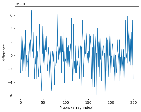
The result is the same using wavecalib and wavecalib_bis (within rounding error).
fig, ax = plt.subplots()
ax.plot(np.sum(data, axis=1)-np.sum(data_wavecalib, axis=1))
ax.set_xlabel('Y axis (array index)')
ax.set_ylabel('difference')
Text(0, 0.5, 'difference')
Graphical Check#
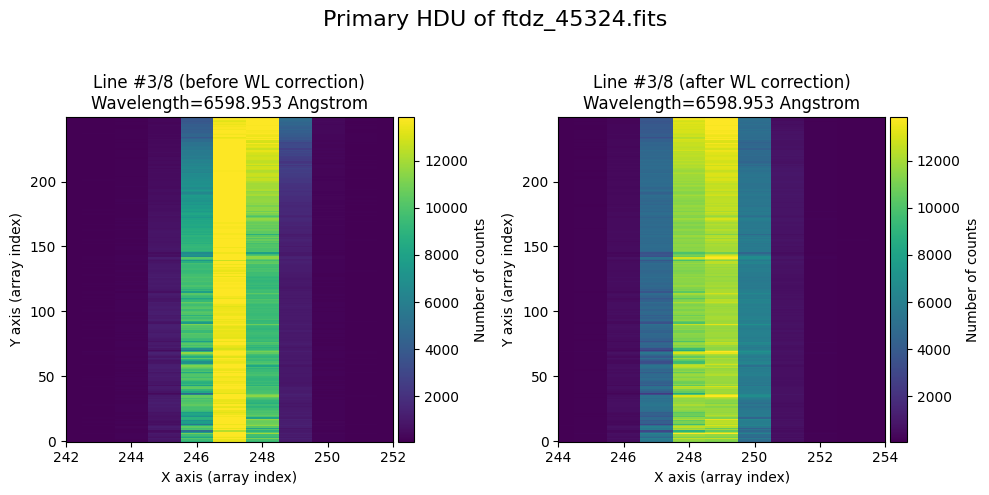
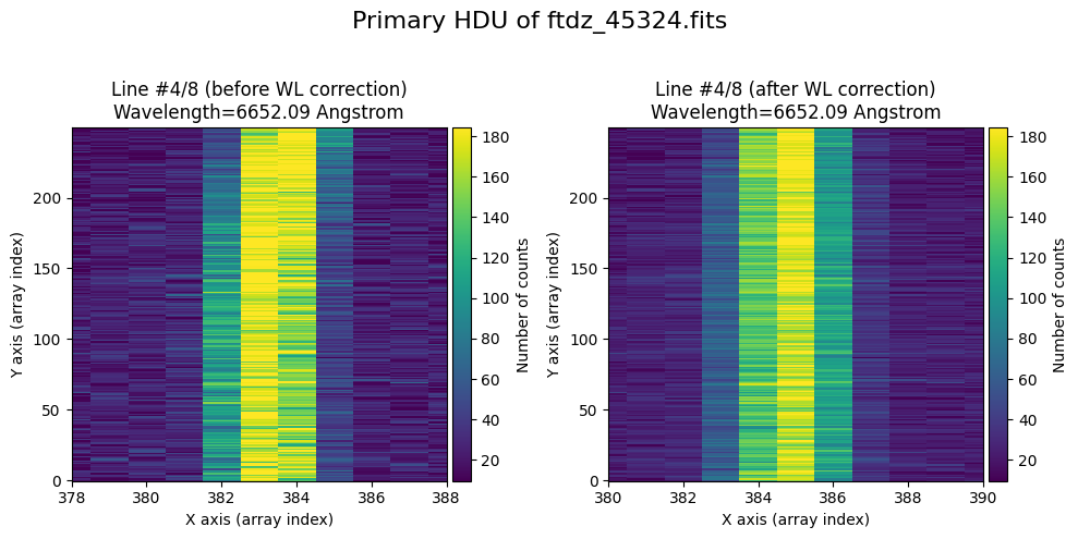
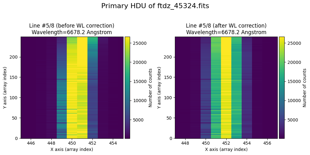
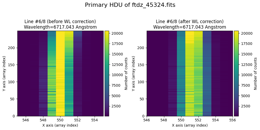
In the vicinity of each line, we will display the image before and after correcting for C distortion and calibrating in wavelength.
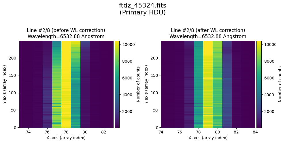
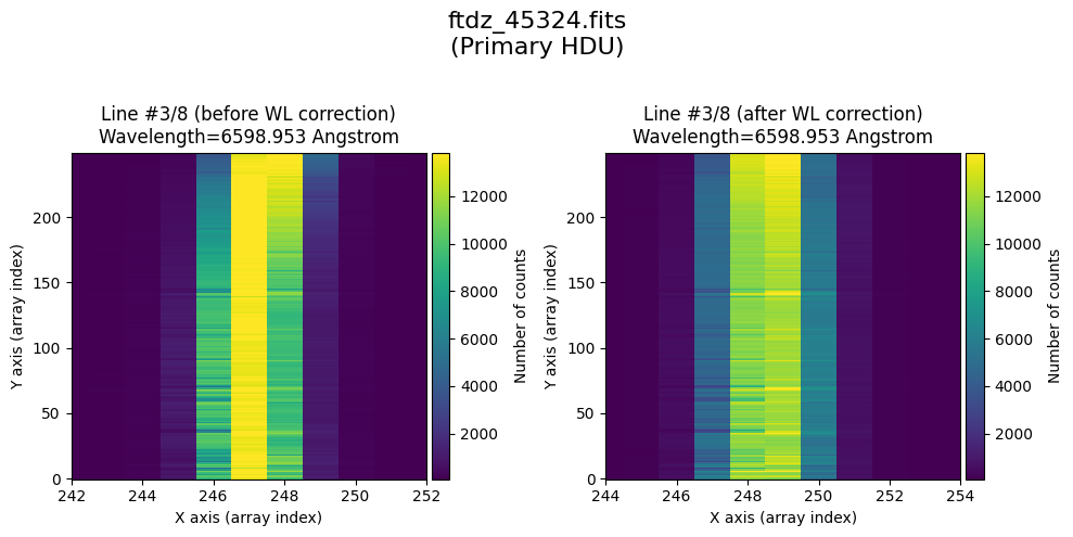
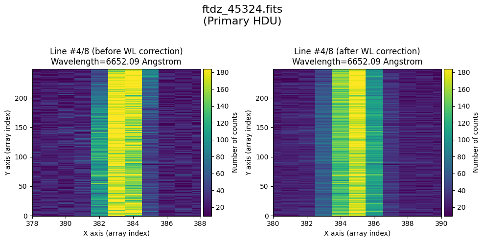
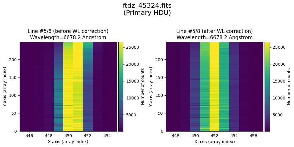
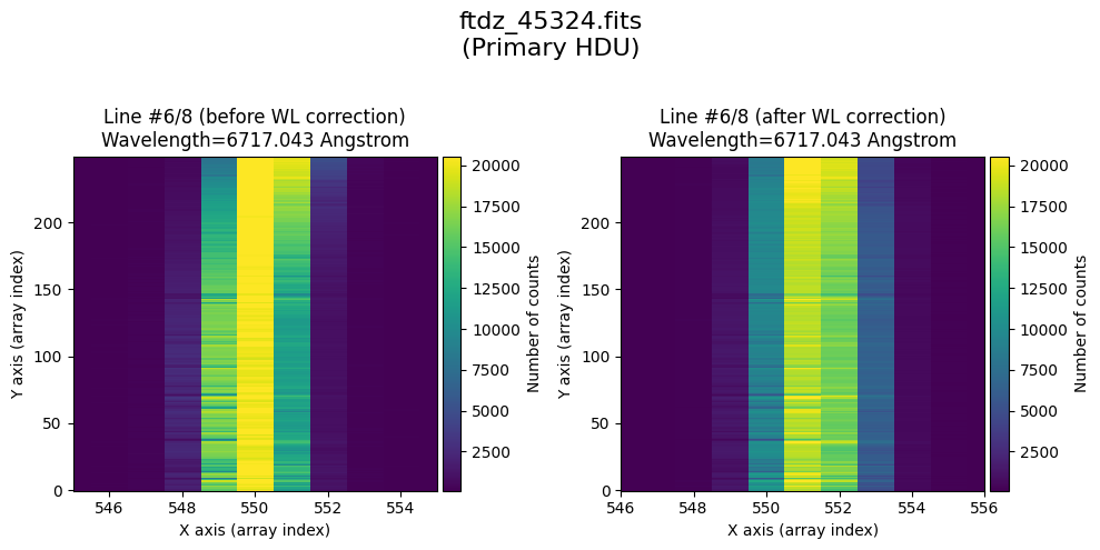
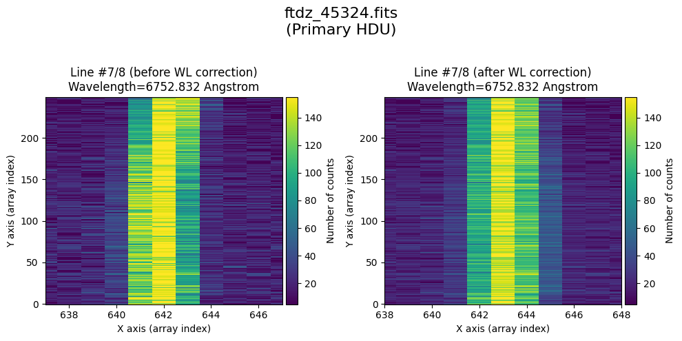
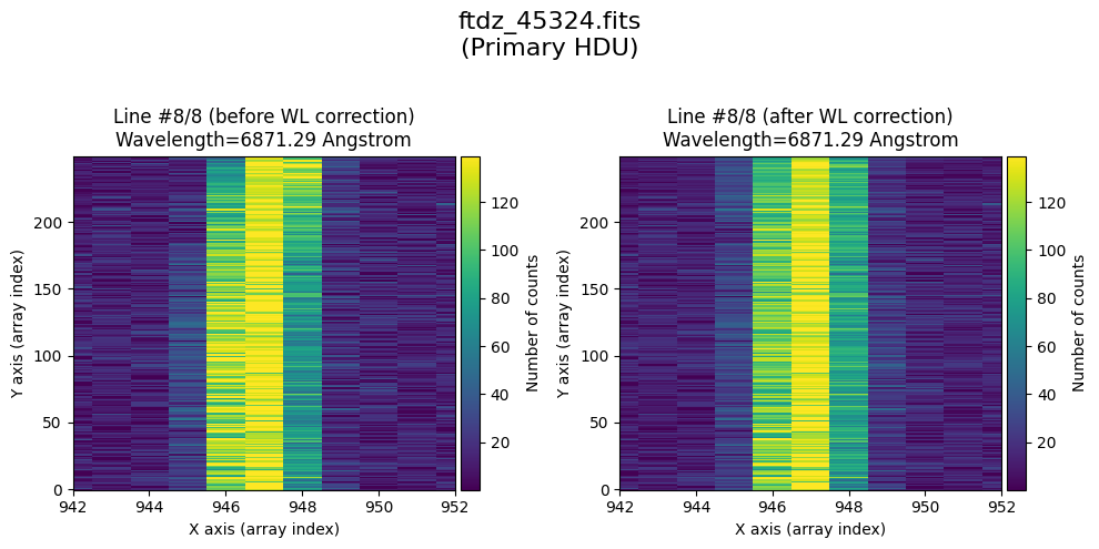
The wavecalib object has a method plot_data_comparison() that graphically represents the image before/after wavelength calibration around each line (the function includes a parameter semi_window, which by default is nx_window, and determines the window, in pixels, to be used).
wavecalib.plot_data_comparison(
    data_before=data,
    data_after=data_wavecalib,
    crval1=crval1,
    cdelt1=cdelt1,
    title=f'Wavelength calibration of {input_filename}'
)
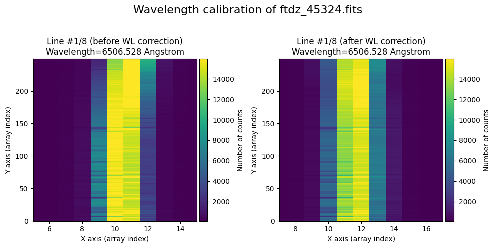

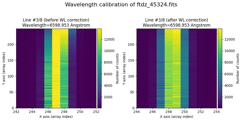
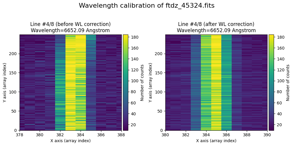
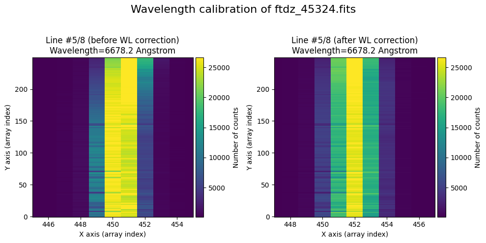
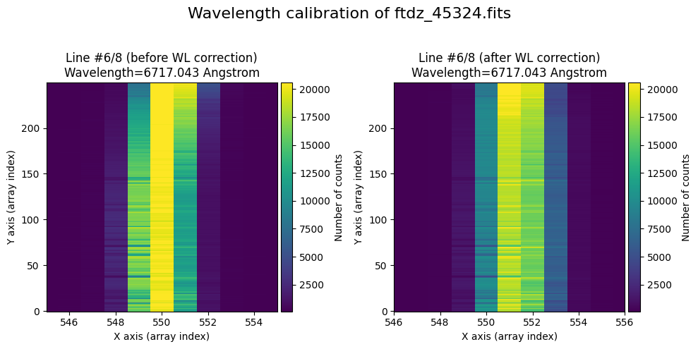
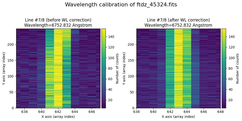
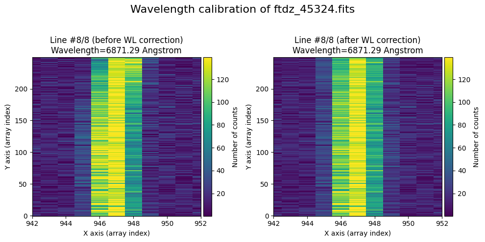
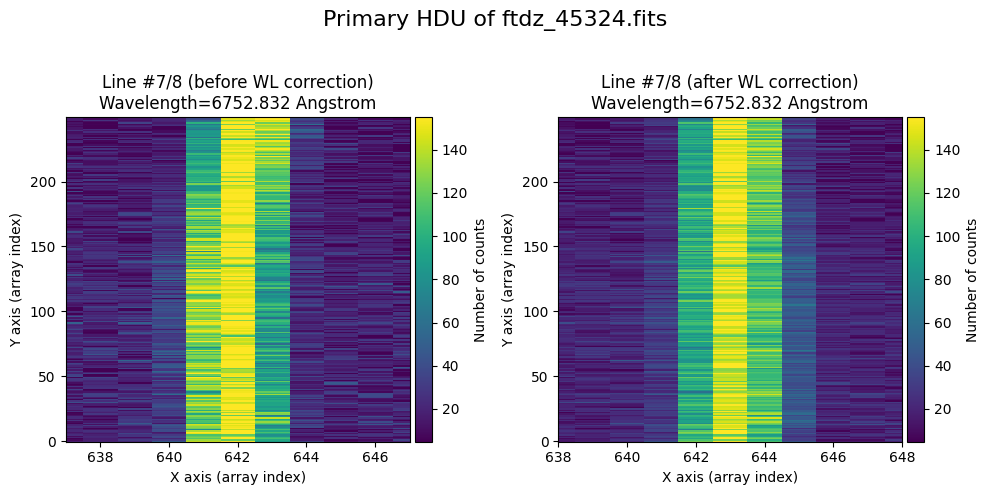
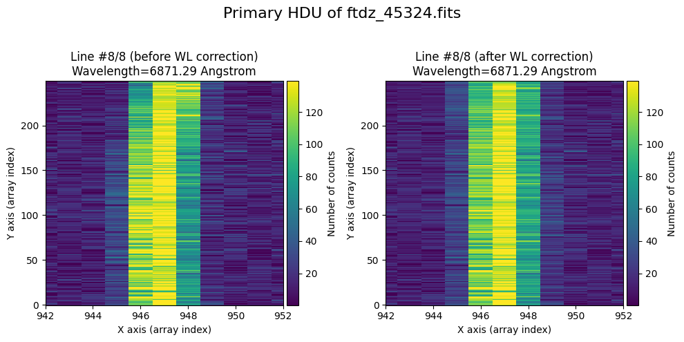
The lines have been straightened: each one shows a slight global shift in the spectral direction (note how the scale on the X-axis changes) due to resampling when converting to a linear wavelength scale.
Numerical Check#
We calibrate in wavelength the image that has already been calibrated. We perform a new calibration process.
wavecalib = tea.TeaWaveCalibration()
wavecalib
TeaWaveCalibration(
    ns_window=11,
    threshold=0,
    sigma_smooth=0,
    nx_window=5,
    delta_flux=0,
    method='gaussian',
    degree_cdistortion=1,
    degree_wavecalib=1,
    peak_wavelengths=None,
    _nlines_reference=None,
    _naxis1=None,
    _naxis2=None,
    _xpeaks_all_lines_array=None,
    _valid_scans=None,
    _list_poly_cdistortion=None,
    _array_poly_wav=None,
    _array_poly_pix=None,
    _array_residual_std_wav=None,
    _array_residual_std_pix=None,
    _array_crval1_linear=None,
    _array_cdelt1_linear=None,
    _array_crmax1_linear=None
)
We use the parameters (threshold, sigma_smooth) that we already know produce a good detection of the relevant peaks.
print(ns_range)
SliceRegion1D(slice(120, 130, None), mode="fits")
xpeaks_reference, ixpeaks_reference, spectrum_reference = wavecalib.compute_xpeaks_reference(
    data=data_wavecalib,
    ns_range=ns_range,
    threshold=50,
    sigma_smooth=2,
    plot_spectrum=True,
    plot_peaks=True
)
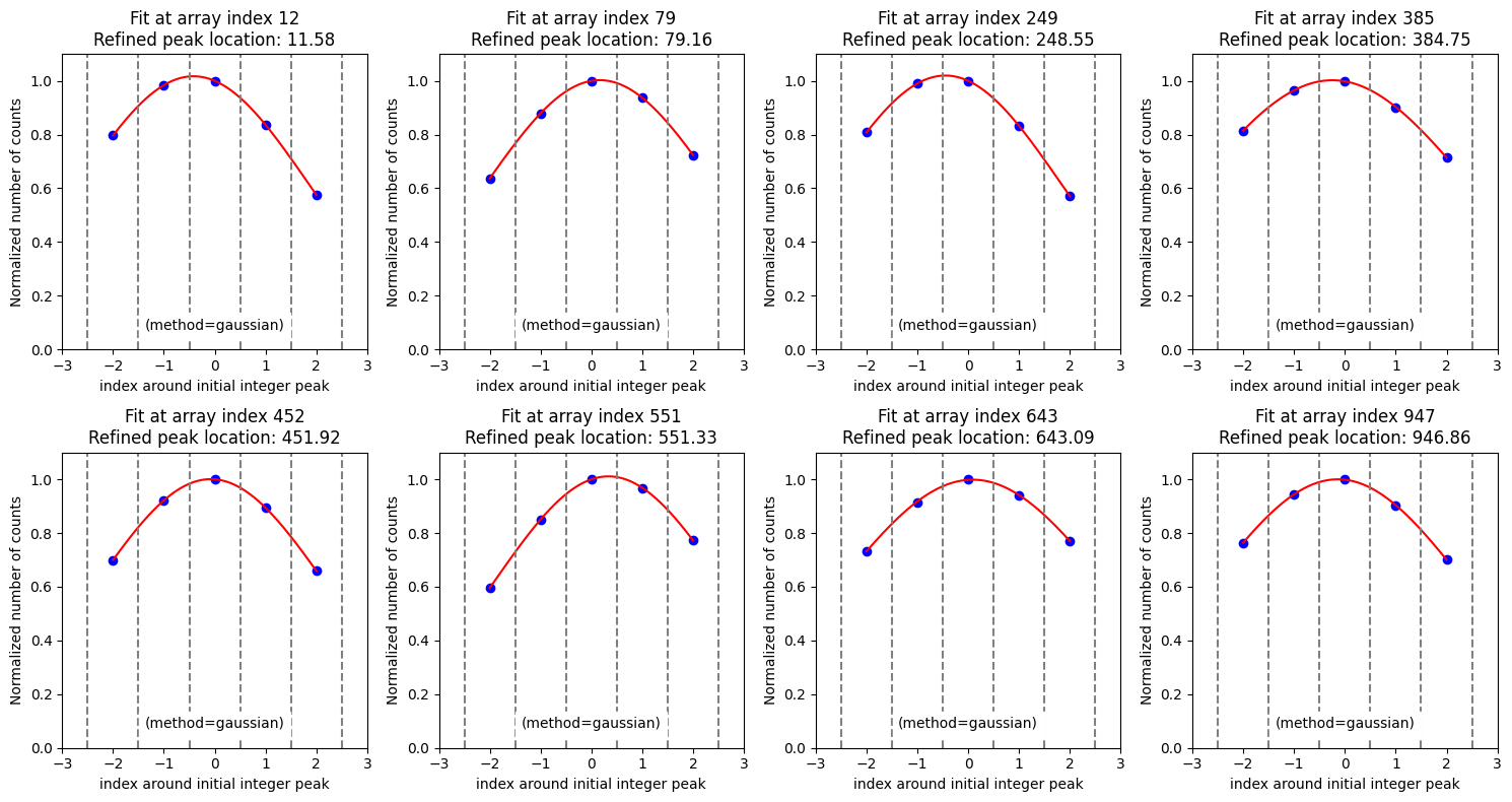
The positions of the peaks and their wavelengths are the same as those used above.
xpeaks_reference
wavelengths_reference
wavecalib.define_peak_wavelengths(
    xpeaks=xpeaks_reference,
    wavelengths= wavelengths_reference
)
We calculate the wavelength calibration polynomial corresponding to the positions of the peaks we have found.
poly_fits_wav, residual_std_wav, poly_fits_pix, residual_std_pix, \
crval1_linear, cdelt1_linear, crmax1_linear = wavecalib.fit_xpeaks_wavelengths(
    xpeaks=xpeaks_reference,
    degree_wavecalib=1,
    debug=True,
    plots=True,
    title=f'Recomputing calibration in calibrated {input_filename}'
)
>>> CRPIX1.............: 1.0 pix
>>> CRVAL1 linear scale: 6502.0075707439155 Angstrom
>>> CDELT1 linear scale: 0.39000734464324466 Angstrom / pix
>>> CRMAX1 linear scale: 6900.985084313955 Angstrom

>>> Fitted coefficients pixel(wavelength):
 [-1.66705003e+04  2.56405428e+00]
>>> Residual std.........................: 0.07231952867883902 pix

>>> Fitted coefficients wavelength(pixel):
 [6.50161756e+03 3.90007345e-01]
>>> Residual std.........................: 0.028205147345884987 Angstrom
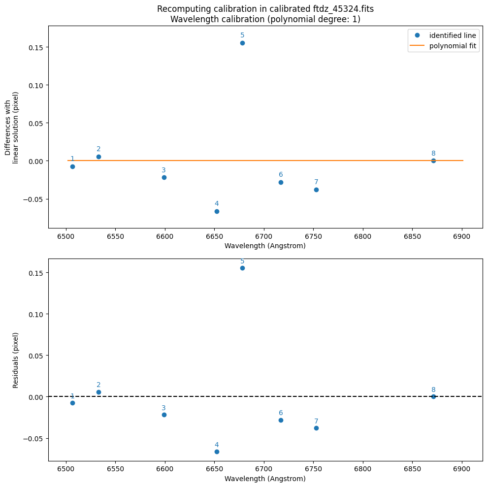
We see that CRVAL1_linear and CDELT1_linear are very close to the values of CRVAL1 and CDELT1 that we used above to obtain the wavelength-calibrated image (which makes sense: the image is already calibrated in wavelength).
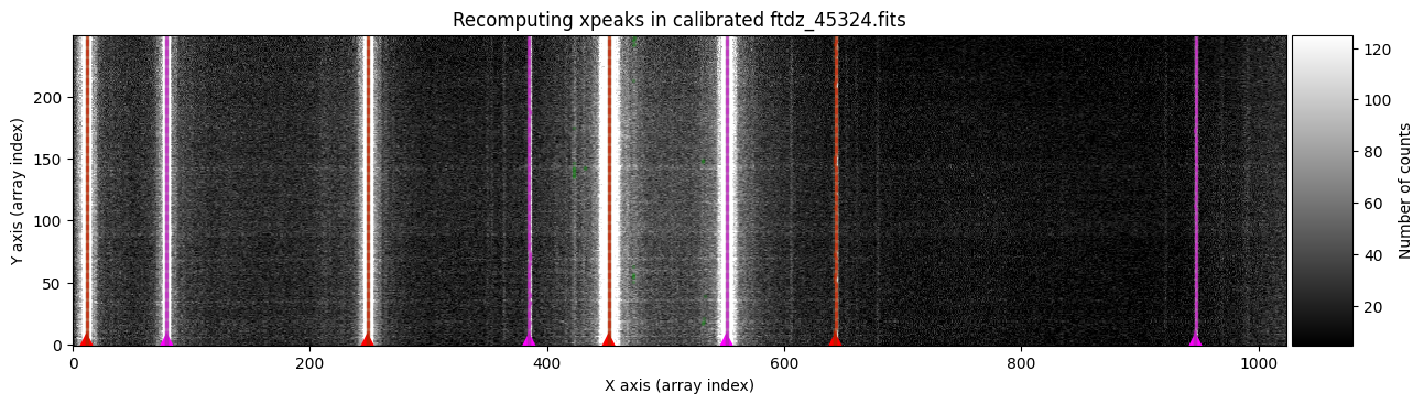
We now proceed to adjust the position of all the lines in the image.
wavecalib.compute_xpeaks_image(
    data=data_wavecalib,
    xpeaks_reference=xpeaks_reference,
    plots=True,
    disable_tqdm=False,
    title=f'Recomputing xpeaks in calibrated {input_filename}'
)
We calculate and adjust the C distortion.
wavecalib.fit_cdistortion(
    plots=True,
    title=f'Recomputing C distortion in calibrated {input_filename}'
)
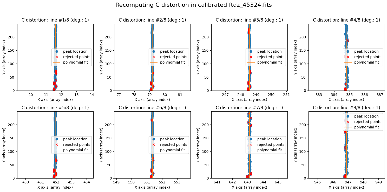
The polynomials obtained are very vertical: there is no noticeable distortion.
wavecalib._list_poly_cdistortion
[Polynomial([1.15930635e+01, 1.28067231e-04], domain=[-1.,  1.], window=[-1.,  1.], symbol='x'),
 Polynomial([ 7.91849325e+01, -2.68337004e-05], domain=[-1.,  1.], window=[-1.,  1.], symbol='x'),
 Polynomial([ 2.48576606e+02, -3.62737522e-05], domain=[-1.,  1.], window=[-1.,  1.], symbol='x'),
 Polynomial([ 3.84823325e+02, -2.06869663e-04], domain=[-1.,  1.], window=[-1.,  1.], symbol='x'),
 Polynomial([4.51944100e+02, 9.84152134e-06], domain=[-1.,  1.], window=[-1.,  1.], symbol='x'),
 Polynomial([ 5.51362468e+02, -5.04764973e-05], domain=[-1.,  1.], window=[-1.,  1.], symbol='x'),
 Polynomial([6.43115049e+02, 3.61309383e-05], domain=[-1.,  1.], window=[-1.,  1.], symbol='x'),
 Polynomial([9.46890352e+02, 7.51850422e-05], domain=[-1.,  1.], window=[-1.,  1.], symbol='x')]
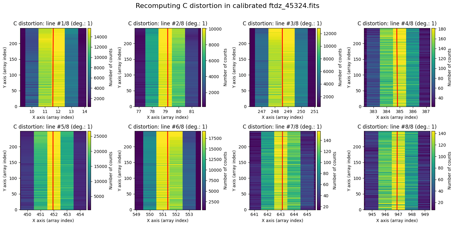
wavecalib.plot_cdistortion(
    data=data_wavecalib,
    title=f'Recomputing C distortion in calibrated {input_filename}'
)
Applying the Calibration to a CCDData Object#
We read the calibration stored in the auxiliary FITS file.
print(wavecal_filename)
wavecal_ftdz_45324.fits
wavecalib = tea.TeaWaveCalibration.read(wavecal_filename)
>>> Reading file.........: wavecal_ftdz_45324.fits
>>> minimum CRVAL1 linear: 6502.280327548579 Angstrom
>>> maximum CRMAX1 linear: 6900.851045180415 Angstrom
>>> mean CDELT1..........: 0.38960969465477574 Angstrom
In case you want to apply this calibration to an instance of type CCDData, it is important to remember that these objects can store different arrays. In particular, the FITS file containing the reduced arc exposure we have been working with contains several extensions.
print(input_filename)
ftdz_45324.fits
fits.info(input_filename)
Filename: ftdz_45324.fits
No.    Name      Ver    Type      Cards   Dimensions   Format
  0  PRIMARY       1 PrimaryHDU     171   (1024, 250)   float64
  1  MASK          1 ImageHDU         8   (1024, 250)   uint8
  2  UNCERT        1 ImageHDU         9   (1024, 250)   float64
We are going to apply the calibration to the 3 present extensions. When doing so on the UNCERT extension, we will introduce uncertainty correlation, which makes its propagation incorrect. In any case, we execute it here to get a first estimate of it.
We read the complete information from the FITS file and generate an instance of type CCDData.
ccdimage = CCDData.read(input_filename)
The mask we have read is completely filled with False values.
ccdimage.mask.any()
np.False_
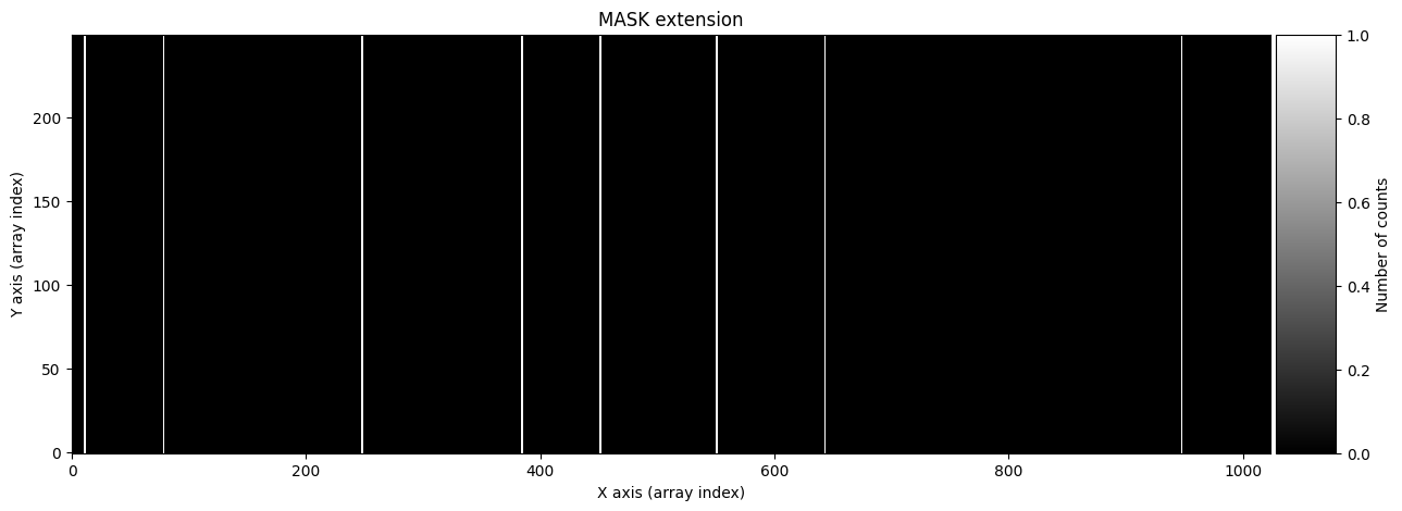
To verify that the calibration is also applied to the mask, we set to True the pixels corresponding to the peaks of the lines (using the prediction from the distortion C calibration polynomials).
for iline in range(wavecalib._nlines_reference):
    indices = (wavecalib._list_poly_cdistortion[iline](range(wavecalib._naxis2))+0.5).astype(int)
    ccdimage.mask[:, indices] = True
We display the mask by converting the boolean array into another one of real numbers, using NumPy’s astype(float) method.
fig, ax = plt.subplots(figsize=(15, 5))
vmin, vmax = 0, 1
img = ax.imshow(ccdimage.mask.astype(float),
                vmin=vmin, vmax=vmax, cmap='gray',
                origin='lower', aspect='auto', interpolation='nearest')
divider = make_axes_locatable(ax)
cax = divider.append_axes("right", size="5%", pad=0.05)
fig.colorbar(img, cax=cax, label='Number of counts')
ax.set_xlabel('X axis (array index)')
ax.set_ylabel('Y axis (array index)')
ax.set_title('MASK extension')
Text(0.5, 1.0, 'MASK extension')
We duplicate the ccdimage object to store in it the result of applying the distortion C correction and the wavelength calibration.
ccdimage_wavecalib = ccdimage.copy()
We apply the distortion C correction and the wavelength calibration to the 3 extensions. In the case of the mask, we first convert it into real numbers, perform the wavelength calibration, and finally store it as a boolean array by setting to True the values greater than zero.
# apply C-distortion correction and wavelength calibration to PRIMARY extension
ccdimage_wavecalib.data = wavecalib.apply(
    data=ccdimage.data,
    crval1=crval1,
    cdelt1=cdelt1,
    disable_tqdm=False
)

# apply C-distortion correction and wavelength calibration to MASK extension
ccdimage_wavecalib.mask = wavecalib.apply(
    data=ccdimage.mask.astype(float),
    crval1=crval1,
    cdelt1=cdelt1,
    disable_tqdm=False
) > 0

# apply C-distortion correction and wavelength calibration to UNCERT extension
ccdimage_wavecalib.uncertainty.array = wavecalib.apply(
    data=ccdimage.uncertainty.array,
    crval1=crval1,
    cdelt1=cdelt1,
    disable_tqdm=False
)
>>> Using CDELT1: 1 pix
>>> Using CRVAL1: 6502.0 Angstrom
>>> Using CDELT1: 0.39 Angstrom / pix
>>> Using CDELT1: 1 pix
>>> Using CRVAL1: 6502.0 Angstrom
>>> Using CDELT1: 0.39 Angstrom / pix
>>> Using CDELT1: 1 pix
>>> Using CRVAL1: 6502.0 Angstrom
>>> Using CDELT1: 0.39 Angstrom / pix
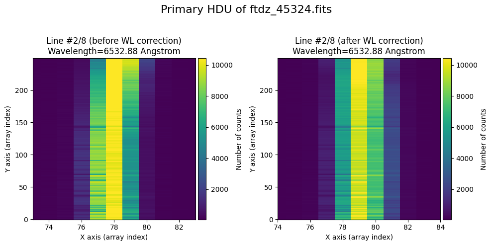
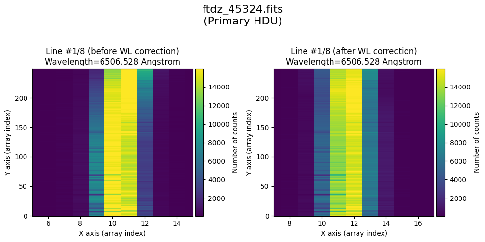
We show the result before / after applying the calibration on the PRIMARY extension.
wavecalib.plot_data_comparison(
    data_before=ccdimage.data,
    data_after=ccdimage_wavecalib.data,
    crval1=crval1,
    cdelt1=cdelt1,
    title=f'Primary HDU of {input_filename}'
)

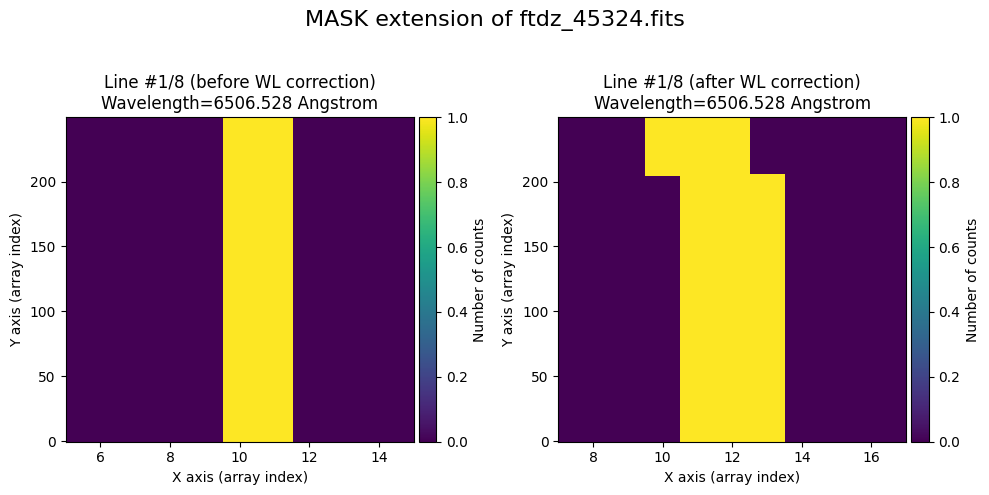
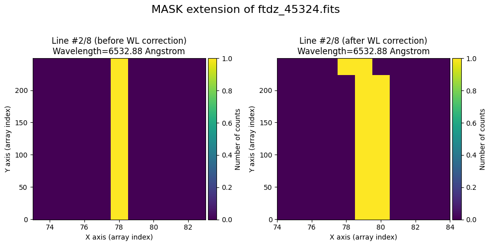
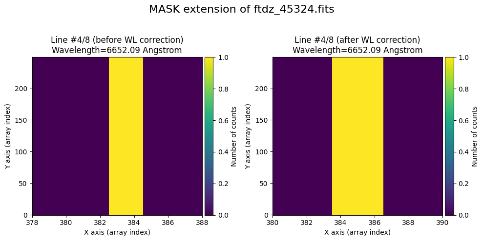
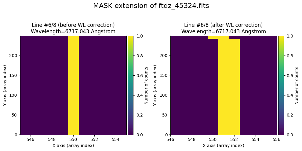
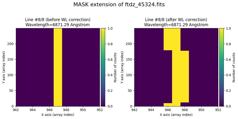
We show the result before / after applying the calibration on the MASK extension.
wavecalib.plot_data_comparison(
    data_before=ccdimage.mask.astype(float),
    data_after=ccdimage_wavecalib.mask.astype(float),
    crval1=crval1,
    cdelt1=cdelt1,
    title=f'MASK extension of {input_filename}'
)


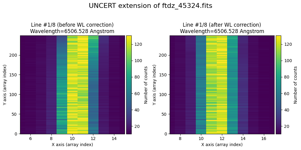
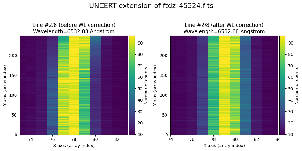
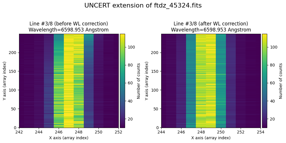
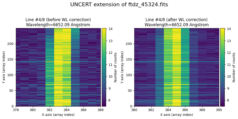
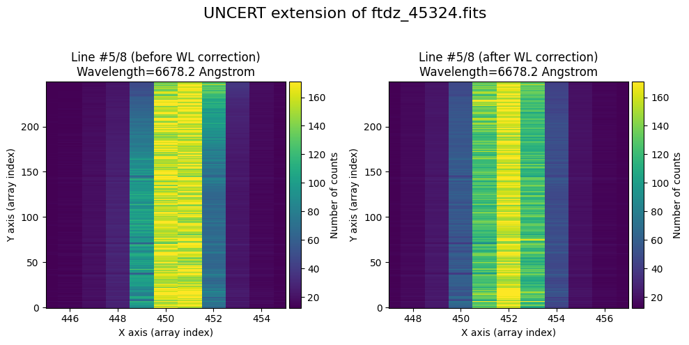
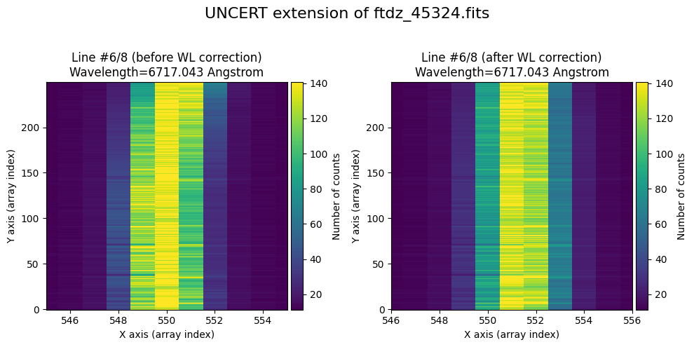
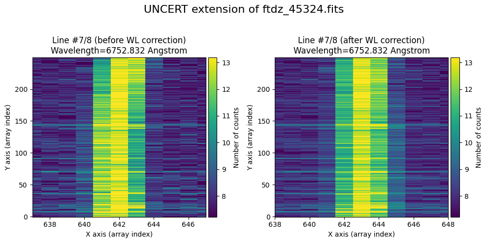
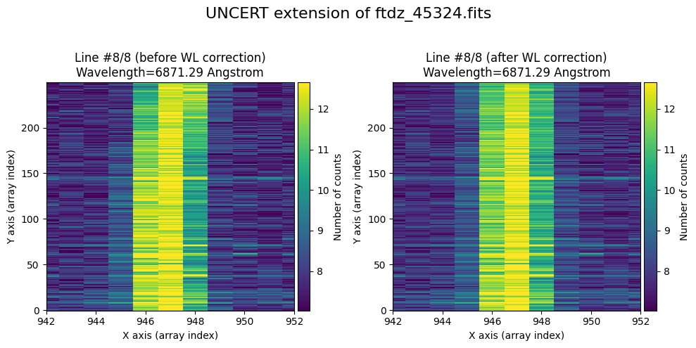
We show the result before / after applying the calibration on the UNCERT extension (we emphasize that from this point on, the errors stored in this array will be correlated).
wavecalib.plot_data_comparison(
    data_before=ccdimage.uncertainty.array,
    data_after=ccdimage_wavecalib.uncertainty.array,
    crval1=crval1,
    cdelt1=cdelt1,
    title=f'UNCERT extension of {input_filename}'
)
We finally save the resulting CCDData object.
# include wavelength calibration parameters
ccdimage_wavecalib.header['CRPIX1'] = (1, f'{u.pixel}')
ccdimage_wavecalib.header['CRVAL1'] = (crval1.value, f'{crval1.unit}')
ccdimage_wavecalib.header['CDELT1'] = (cdelt1.value, f'{cdelt1.unit}' )
ccdimage_wavecalib.header['CUNIT1'] = (f'{crval1.unit}', 'wavelength unit')
ccdimage_wavecalib.header['CTYPE1'] = ('AWAV', 'air wavelength')

# update FILENAME keyword with output file name
output_filename = f'w{input_filename}'
ccdimage_wavecalib.header['FILENAME'] = output_filename
# update HISTORY in header
ccdimage_wavecalib.header['HISTORY']  = '-------------------'
ccdimage_wavecalib.header['HISTORY']  = f"{datetime.now().strftime('%Y-%m-%d %H:%M:%S')}"
ccdimage_wavecalib.header['HISTORY'] = 'using tea_wavecal'
ccdimage_wavecalib.header['HISTORY'] = f'calibration file: {wavecal_filename}'

# save result
ccdimage_wavecalib.write(output_filename, overwrite='yes')
print(f'Output file name.: {output_filename}')
Output file name.: wftdz_45324.fits
Auxiliary function apply_wavecal_ccddata()#
We have defined an auxiliary function called apply_wavecal_ccddata() that facilitates the application of wavelength calibration on FITS files that store CCDData objects.
For example, we can calibrate the previous image, stored in
print(input_filename)
ftdz_45324.fits
using the wavelength calibration stored in
print(wavecal_filename)
wavecal_ftdz_45324.fits
and saving the result in
output_filename = f'ww{input_filename}'
print(output_filename)
wwftdz_45324.fits
We will use the following parameters for the calibrated image:
print(crval1)
print(cdelt1)
6502.0 Angstrom
0.39 Angstrom / pix
The function apply_wavecal_ccdata() is executed easily by including the above information
tea.apply_wavecal_ccddata(
    infile=input_filename,
    wcalibfile=wavecal_filename,
    outfile=output_filename,
    crval1=crval1,
    cdelt1=cdelt1
)
By default, the function runs in “silent” mode (without displaying informational messages), so if we need to apply it automatically to many images, it won’t generate too many messages. If preferred, we can get some feedback by setting silent_mode=False.
tea.apply_wavecal_ccddata(
    infile=input_filename,
    wcalibfile=wavecal_filename,
    outfile=output_filename,
    crval1=crval1,
    cdelt1=cdelt1,
    silent_mode=False
)
>>> Reading file.........: wavecal_ftdz_45324.fits
>>> minimum CRVAL1 linear: 6502.280327548579 Angstrom
>>> maximum CRMAX1 linear: 6900.851045180415 Angstrom
>>> mean CDELT1..........: 0.38960969465477574 Angstrom

>>> Reading file.........: ftdz_45324.fits

Applying calibration to primary HDU
>>> Using CDELT1: 1 pix
>>> Using CRVAL1: 6502.0 Angstrom
>>> Using CDELT1: 0.39 Angstrom / pix
Applying calibration to MASK extension
>>> Using CDELT1: 1 pix
>>> Using CRVAL1: 6502.0 Angstrom
>>> Using CDELT1: 0.39 Angstrom / pix
Applying calibration to UNCERT extension
>>> Using CDELT1: 1 pix
>>> Using CRVAL1: 6502.0 Angstrom
>>> Using CDELT1: 0.39 Angstrom / pix
--> Output FITS file.....: wwftdz_45324.fits
We can also indicate that a graphical comparison is shown before / after running the calibration, using the parameter plot_data_comparison, which can take 3 values:
0: draws nothing
1: compares the data arrays (primary extension)
2: compares the primary HDU and the two extensions (
MASKandUNCERT)
tea.apply_wavecal_ccddata(
    infile=input_filename,
    wcalibfile=wavecal_filename,
    outfile=output_filename,
    crval1=crval1,
    cdelt1=cdelt1,
    silent_mode=False,
    plot_data_comparison=1,
    title=input_filename
)
>>> Reading file.........: wavecal_ftdz_45324.fits
>>> minimum CRVAL1 linear: 6502.280327548579 Angstrom
>>> maximum CRMAX1 linear: 6900.851045180415 Angstrom
>>> mean CDELT1..........: 0.38960969465477574 Angstrom

>>> Reading file.........: ftdz_45324.fits

Applying calibration to primary HDU
>>> Using CDELT1: 1 pix
>>> Using CRVAL1: 6502.0 Angstrom
>>> Using CDELT1: 0.39 Angstrom / pix
Applying calibration to MASK extension
>>> Using CDELT1: 1 pix
>>> Using CRVAL1: 6502.0 Angstrom
>>> Using CDELT1: 0.39 Angstrom / pix
Applying calibration to UNCERT extension
>>> Using CDELT1: 1 pix
>>> Using CRVAL1: 6502.0 Angstrom
>>> Using CDELT1: 0.39 Angstrom / pix
--> Output FITS file.....: wwftdz_45324.fits
* Comparing primary HDU data before / after calibration
time_end = datetime.now()
tea.elapsed_time(time_ini, time_end)
system...........: Darwin
release..........: 25.2.0
machine..........: arm64
node.............: iblax.fis.ucm.es
Python executable: /Users/cardiel/venv_tea/bin/python3.13
teareduce version: 0.7.1
Initial time.....: 2026-02-06 10:27:24.925880
Final time.......: 2026-02-06 10:27:36.726604
Elapsed time.....: 0:00:11.800724