Automatic Cosmic Ray Removal in Double Exposures

This notebook presents the function cr2images(), an alternative approach to tea-cleanest for cleaning cosmic rays in pairs of images.

This code simply computes the difference between the two available images and identifies cosmic ray-affected pixels as those whose difference exceeds the global median by a certain threshold (a multiple of the robust standard deviation).

The function cr2images() replaces the information in pixels suspected of having been affected by cosmic rays using the information from the other image.

The code allows for correction of small offsets between the exposures involved.

from astropy.io import fits
from astropy.nddata import CCDData
from datetime import datetime
import matplotlib.pyplot as plt
import numpy as np
from pathlib import Path
import teareduce as tea

time_ini = datetime.now()
print(time_ini)

2026-01-27 04:39:35.291492

Download the required files

for fname in [
    'notebooks/cr2images/ftdz_45243.fits',
    'notebooks/cr2images/ftdz_45244.fits'
]:
    tea.get_cookbook_file(fname)

File ftdz_45243.fits already exists locally. Skipping download.

File ftdz_45244.fits already exists locally. Skipping download.

tea.avoid_astropy_warnings(True)

Cosmic Ray Detection Using Equivalent Exposures

When two equivalent exposures are available (same exposure time, similar background and object signal, and identical pointing), cosmic rays can be detected by subtracting one image from the other. If the background signal differs between the images, the strategy described below can still be applied, considering that the average value of the difference may be non-zero.

Additionally, if the two images are offset by an integer number of pixels, one image can be shifted and the cosmic ray cleaning process can be performed using only the overlapping region of the two exposures.

The cosmic ray detection process proceeds as follows:

1. Assume the two arrays are stored in data1 and data2.

2. Subtract the images: diff = data1 - data2. Cosmic rays in the first image will appear as very bright pixels (strong positive signal), while those in the second image will appear as very dark pixels (strong negative signal).

3. Compute the global median and robust standard deviation of diff.

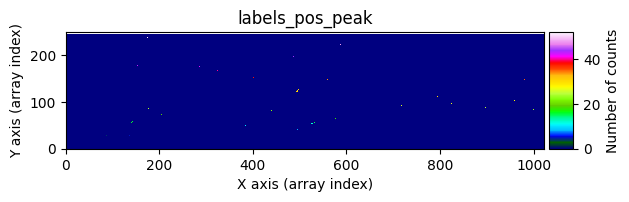
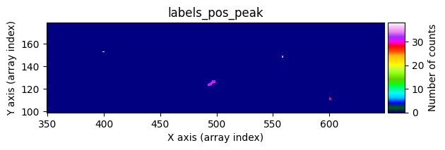
4. Identify cosmic ray-affected pixels as those whose signal exceeds the image median by a certain threshold (a multiple of the robust standard deviation). This can be done using scipy.ndimage.label(), which not only detects the affected pixels but also labels them with unique identifiers. Connected pixel structures receive the same label. This results in an array labels_pos_peak (where pos indicates positive values and peak refers to the brightest pixels).

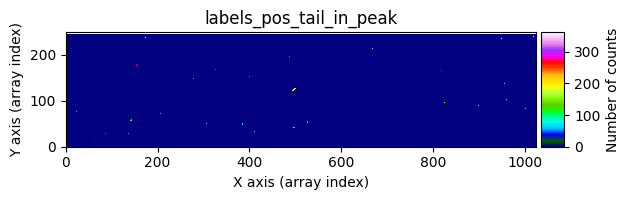
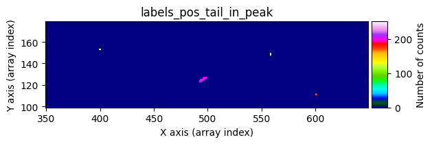
5. Detect neighboring pixels that may also be affected by cosmic rays using a less strict threshold. This produces an array labels_pos_tail (tail refers to the “tails” of cosmic rays, i.e., affected pixels with lower signal).

6. Convert labels_pos_peak to a binary mask mask_pos_peak (containing only 0s and 1s), where any pixel in labels_pos_peak with a value greater than zero is set to 1.

7. Multiply mask_pos_peak by labels_pos_tail to obtain an array labels_pos_tail_in_peak, which contains the labels from labels_pos_tail corresponding to objects detected in labels_pos_peak.

8. Generate a binary mask mask_pos_clean, where pixels in labels_pos_tail whose labels appear in labels_pos_tail_in_peak are set to 1. This mask indicates which pixels need to be corrected.

9. Replace the affected pixels in data1 with the corresponding values from data2 using mask_pos_clean. If the selected pixels in data2 are also affected by cosmic rays, the correction will fail, but the probability of this is low.

10. Repeat the process for the second image, swapping data1 and data2 (i.e., compute diff = data2 - data1) and follow the same steps to detect and correct cosmic rays in data2.

All of the above steps are implemented in the auxiliary function cr2images() defined in the teareduce package. Users only need to call this function to perform the cleaning.

Using cr2images()

We will test the functionality of this function using the two available exposures of the galaxy UCM1256+2701.

input_filename1 = 'ftdz_45243.fits'
input_filename2 = 'ftdz_45244.fits'

We read the headers and data from the two exposures and verify that they correspond to the same object and have the same exposure time.

header1 = fits.getheader(input_filename1)
data1 = fits.getdata(input_filename1)

header2 = fits.getheader(input_filename2)
data2 = fits.getdata(input_filename2)

print(header1['OBJECT'])
print(header2['OBJECT'])

print(header1['EXPTIME'])
print(header2['EXPTIME'])

U1256+2701 PA=300
U1256+2701 PA=300
600.0
600.0

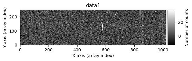
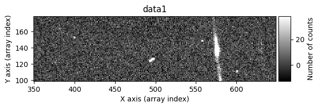
We display the two images to visually compare them.

vmin, vmax = np.percentile(data1, [0, 99.9])

for data, header in zip([data1, data2], [header1, header2]):
    fig, ax = plt.subplots(figsize=(15, 5))
    tea.imshow(fig, ax, data, vmin=vmin, vmax=vmax)
    ax.set_title(f'{header["OBJECT"]}: {header["FILENAME"]},  EXPTIME={header["EXPTIME"]}')
    plt.show()

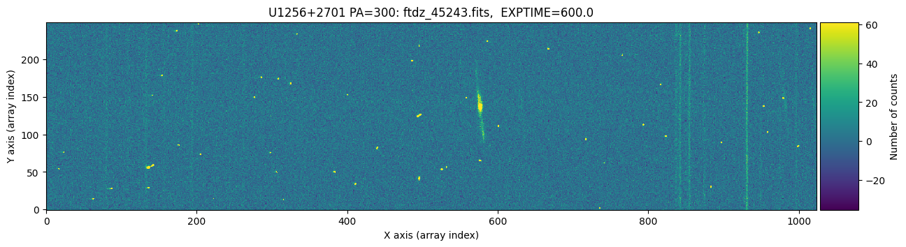
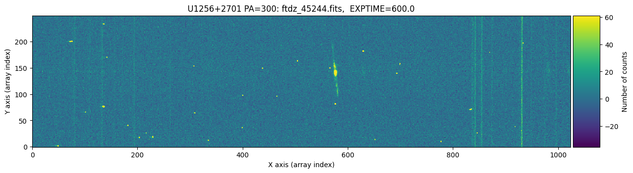
The images appear to have the same pointing. We zoom in slightly on the bright emission line and adjust the display scaling to better detect the peak of the line.

fig, axarr = plt.subplots(nrows=1, ncols=2, figsize=(10, 5))
for iplot, (data, header) in enumerate(zip([data1, data2], [header1, header2])):
    ax = axarr[iplot]
    tea.imshow(fig, ax, data, vmin=-30, vmax=130)
    ax.set_title(f'{header["FILENAME"]}')
    ax.set_xlim([562, 588])
    ax.set_ylim([125, 150])
plt.tight_layout()

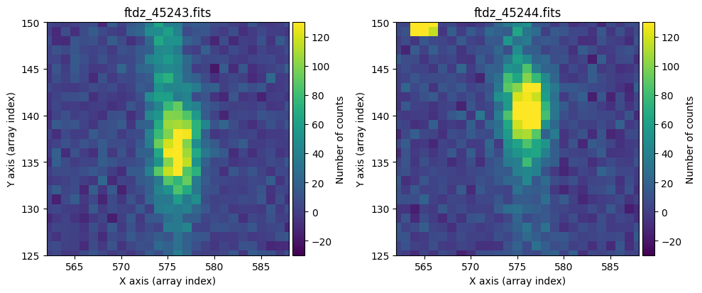
We can see that there is no offset along the X-axis, but there is along the vertical axis: the image on the right appears 4 pixels higher. This is something to keep in mind.

We can run cr2images() by specifying:

• The arrays to be cleaned: data1 and data2.

• The offsets ioffx, ioffy: these must be integers, representing the shift needed to align data2 with data1.

• The thresholds for detecting cosmic ray peaks and tails: tsigma_peak and tsigma_tail. These indicate how many times the robust standard deviation above the image median is used to classify a pixel as a cosmic ray.

When executed with these parameters (and no others), the function returns the two arrays cleaned of cosmic rays (referred to here as data1c and data2c).

data1c, data2c = tea.cr2images(
    data1=data1,
    data2=data2,
    ioffx=0,
    ioffy=-4,
    tsigma_peak=10,
    tsigma_tail=3
)

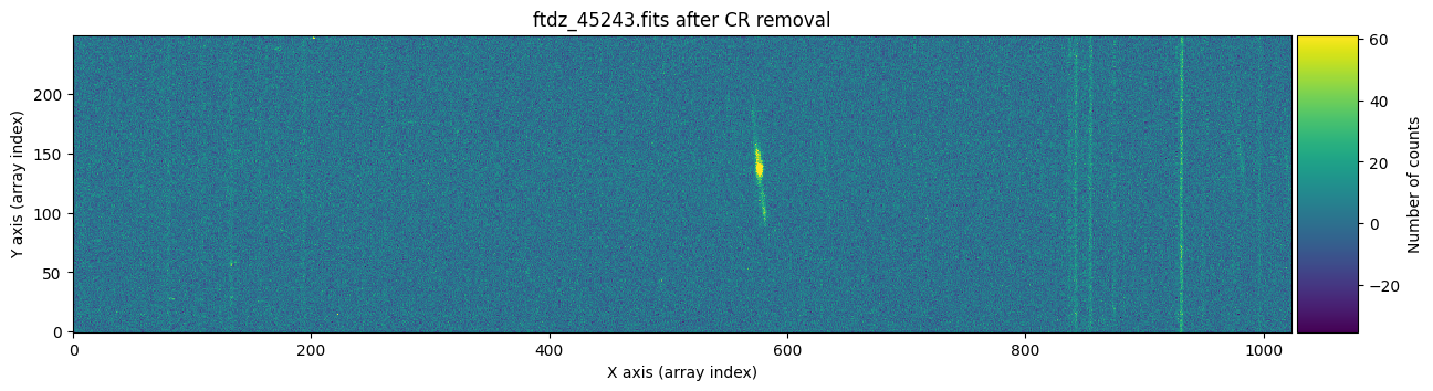
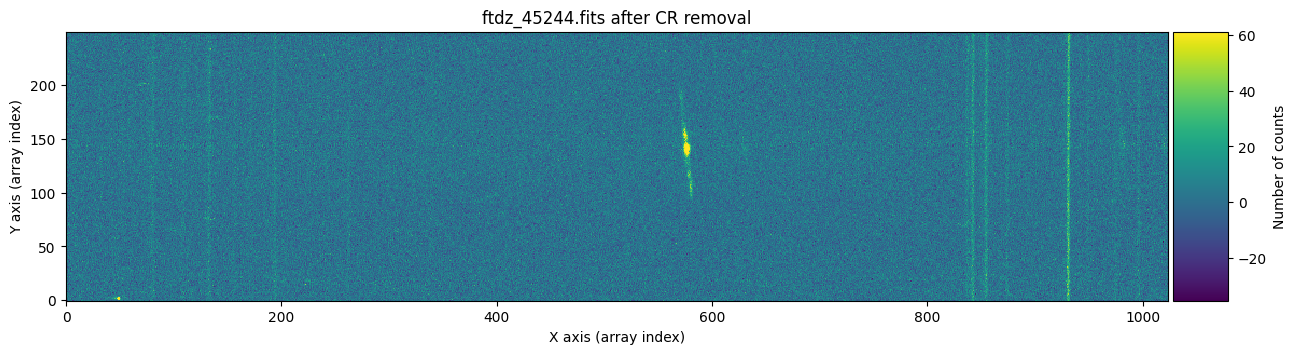
We check the result of cleaning the first image.

vmin, vmax = np.percentile(data1, [0, 99.9])

for data, header, when in zip([data1, data1c], 
                              [header1, header1], 
                              ['before', 'after']):
    fig, ax = plt.subplots(figsize=(15, 5))
    tea.imshow(fig, ax, data, vmin=vmin, vmax=vmax)
    ax.set_title(f'{header["FILENAME"]} {when} CR removal')
    plt.show()

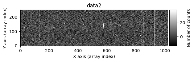
And now we show the second image before and after cleaning the cosmic rays.

vmin, vmax = np.percentile(data2, [0, 99.9])

for data, header, when in zip([data2, data2c], 
                              [header2, header2], 
                              ['before', 'after']):
    fig, ax = plt.subplots(figsize=(15, 5))
    tea.imshow(fig, ax, data, vmin=vmin, vmax=vmax)
    ax.set_title(f'{header["FILENAME"]} {when} CR removal')
    plt.show()

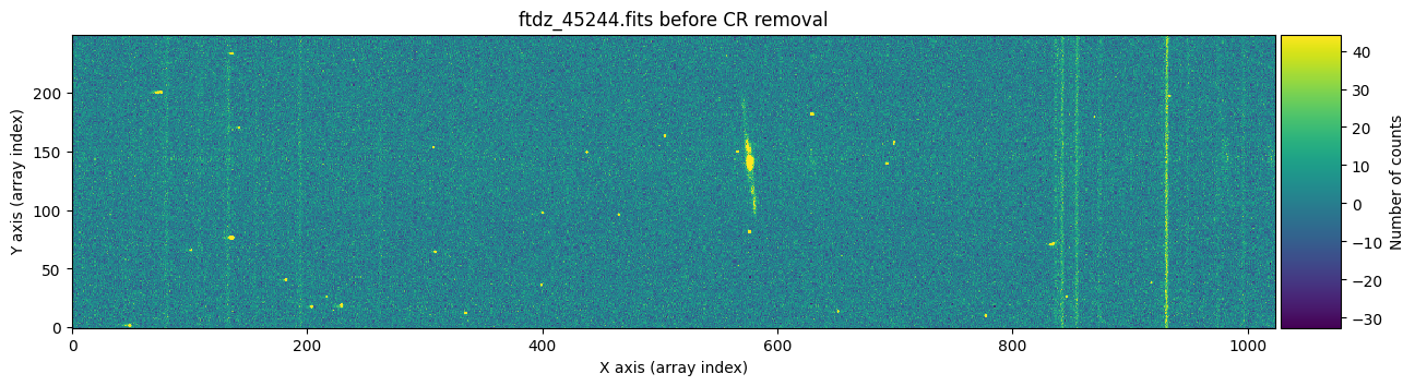
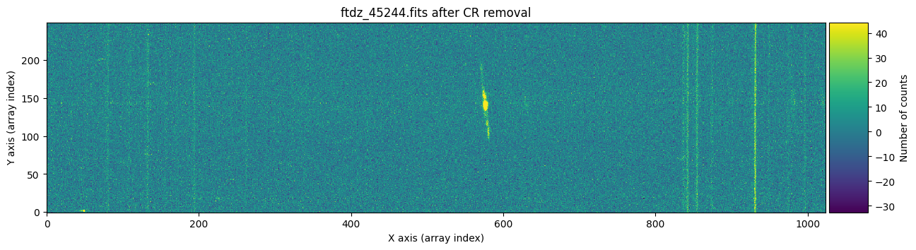
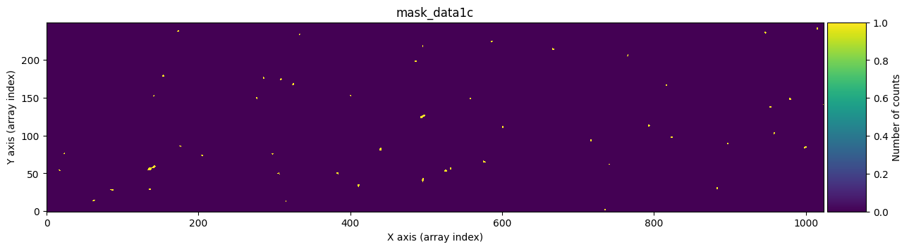
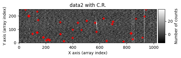
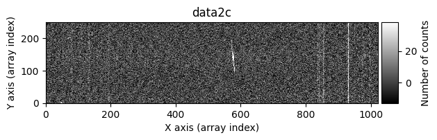
Apparently, the images have been well cleaned. However, we might still wonder whether any signal from the object has been removed, for example in the region of the bright emission line. To find out which pixels were corrected in each case, we can run cr2images() specifying that we want to obtain a mask with the positions of the pixels affected by cosmic rays. To do this, we need to use the parameter return_masks=True, and keep in mind that the function call now returns four objects.

data1c, data2c, mask_data1c, mask_data2c = tea.cr2images(
    data1=data1,
    data2=data2,
    ioffx=0,
    ioffy=-4,
    tsigma_peak=10,
    tsigma_tail=3,
    return_masks=True
)

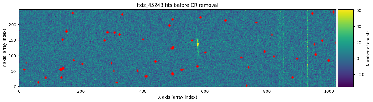
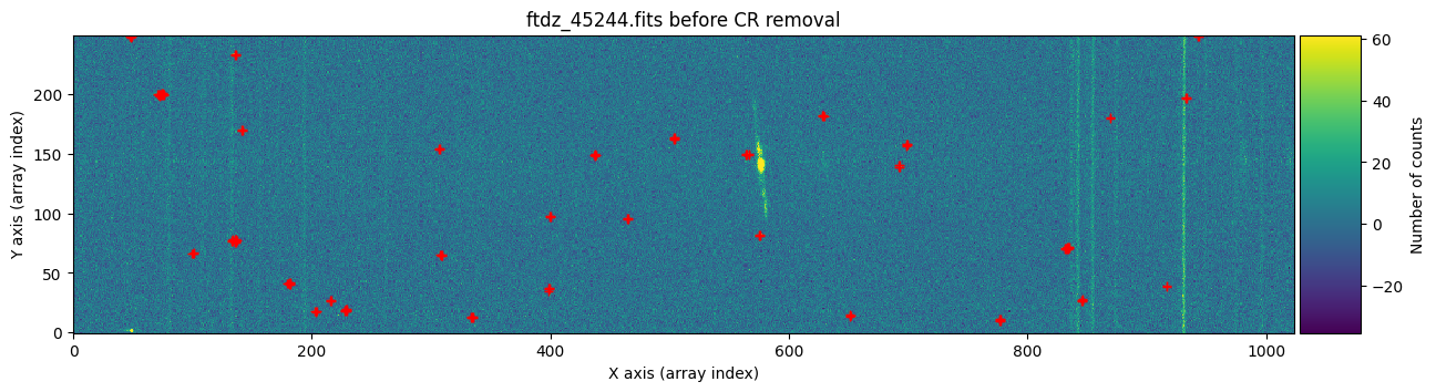
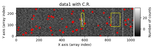
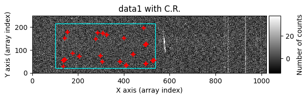
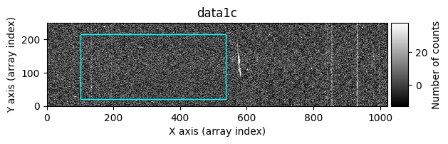
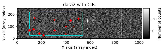
We draw the first image again, this time three times: before cleaning, before cleaning with red crosses marking the detected cosmic rays, and after cleaning.

vmin, vmax = np.percentile(data1, [0, 99.9])

for data, header, when, overplot_mask in zip([data1, data1, data1c], 
                                             [header1, header1, header1], 
                                             ['before', 'before', 'after'],
                                             [False, True, False]):
    fig, ax = plt.subplots(figsize=(15, 5))
    tea.imshow(fig, ax, data, vmin=vmin, vmax=vmax)
    if overplot_mask:
        xyp = np.argwhere(mask_data1c > 0)
        xp = [item[1] for item in xyp]
        yp = [item[0] for item in xyp]
        ax.plot(xp, yp, 'r+')
    ax.set_title(f'{header["FILENAME"]} {when} CR removal')
    plt.show()

We repeat the same procedure with the second image.

vmin, vmax = np.percentile(data1, [0, 99.9])

for data, header, when, overplot_mask in zip([data2, data2, data2c], 
                                             [header2, header2, header2], 
                                             ['before', 'before', 'after'],
                                             [False, True, False]):
    fig, ax = plt.subplots(figsize=(15, 5))
    tea.imshow(fig, ax, data, vmin=vmin, vmax=vmax)
    if overplot_mask:
        xyp = np.argwhere(mask_data2c > 0)
        xp = [item[1] for item in xyp]
        yp = [item[0] for item in xyp]
        ax.plot(xp, yp, 'r+')
    ax.set_title(f'{header["FILENAME"]} {when} CR removal')
    plt.show()

To find out whether a cosmic ray hit the same pixel in both exposures, it is enough to multiply the two masks and check if there is any overlap.

mask_product = mask_data1c * mask_data2c
mask_product.any()

np.False_

False indicates that there has been no overlap.

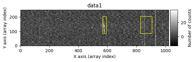
Selecting Regions to Clean

The cr2images() function allows:

• Option 1: specify regions that should not be cleaned of cosmic rays (using a list of rectangular regions). This is useful when we want to prevent certain areas from being mistakenly corrected. To use this option, you must use the list_skipped_regions parameter, which should be a Python list containing objects of type SliceRegion2D.

• Option 2: specify the region to be cleaned (rectangular region). This allows cosmic ray removal to be performed in specific areas of the image. To choose this approach, you must use the image_region parameter, which should be a single object of type SliceRegion2D.

The two options above are mutually exclusive (you can choose one or the other, but not both at the same time). Let’s look at both possibilities in practice.

Option 1: Using list_skipped_regions

We start by excluding a series of regions. For convenience, cr2images() can also display the images before and after cleaning the cosmic rays. This option is activated by using debug_level=1.

list_skipped_regions = [
    tea.SliceRegion2D(np.s_[568:594, 85:205], mode='fits'),
    tea.SliceRegion2D(np.s_[829:909, 85:205], mode='fits'),
]

data1c, data2c, mask_data1c, mask_data2c = tea.cr2images(
    data1=data1,
    data2=data2,
    ioffx=0,
    ioffy=-4,
    tsigma_peak=10,
    tsigma_tail=3,
    list_skipped_regions=list_skipped_regions,
    return_masks=True,
    debug_level=1
)

Computing overlaping rectangle:
ioffx: 0
ioffx: -4
data1:  i1,  i2,  j1,  j2: 0, 246, 0, 1024
data2: ii1, ii2, jj1, jj2: 4, 250, 0, 1024
shape1: (246, 1024), shape2: (246, 1024), shape(diff): (246, 1024)

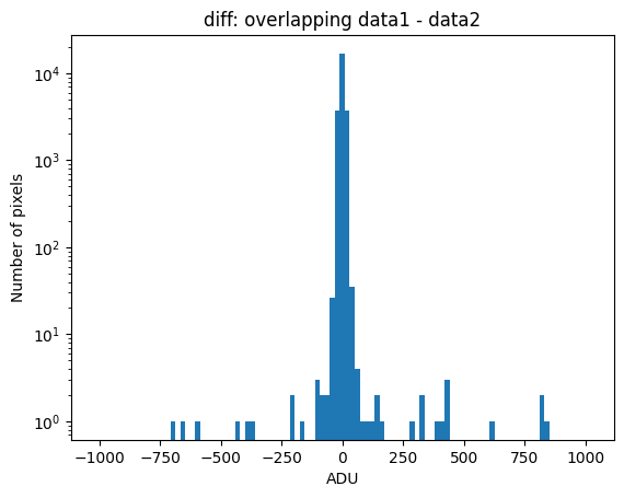
>>> Statistical summary of diff = overlapping data1 - data2:
>>> Median....: -0.179
>>> Robust_std: 10.149
>>> Searching for positive peaks (CR in data1) with tsigma_peak=10
>>> Found 52 positive peaks
>>> Searching for positive tails (CR in data1) with tsigma_tail=3
>>> Found 371 positive tails
>>> Merging positive peaks and tails
>>> Replacing 276 pixels affected by cosmic rays in data1
>>> Finished replacing pixels affected by cosmic rays in data1
>>> Searching for negative peaks (CR in data2) with tsigma_peak=10
>>> Found 31 negative peaks
>>> Searching for negative tails (CR in data2) with tsigma_tail=3
>>> Found 405 negative tails
>>> Merging negative peaks and tails
>>> Replacing 173 pixels affected by cosmic rays in data2
>>> Finished replacing pixels affected by cosmic rays in data2
Number of CR in data1: 52 peaks, 371 tails

Number of CR in data2: 31 peaks, 405 tails

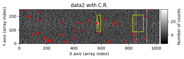
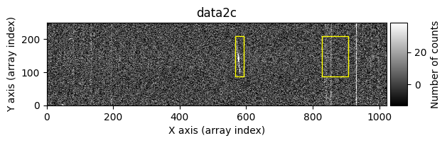
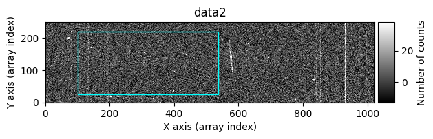
The yellow rectangles indicate regions where the removal of potential cosmic rays was not allowed.

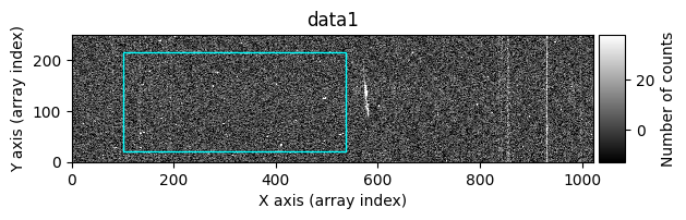
Option 2: Using image_region

In the following execution, we will specify that we want to clean only a specific region of the image:

data1c, data2c, mask_data1c, mask_data2c = tea.cr2images(
    data1=data1,
    data2=data2,
    ioffx=0,
    ioffy=-4,
    tsigma_peak=10,
    tsigma_tail=3,
    image_region=tea.SliceRegion2D(np.s_[102:539, 22:217], mode='fits'),
    return_masks=True,
    debug_level=1
)

Computing overlaping rectangle:
ioffx: 0
ioffx: -4
data1:  i1,  i2,  j1,  j2: 0, 246, 0, 1024
data2: ii1, ii2, jj1, jj2: 4, 250, 0, 1024
shape1: (246, 1024), shape2: (246, 1024), shape(diff): (246, 1024)

>>> Statistical summary of diff = overlapping data1 - data2:
>>> Median....: -0.179
>>> Robust_std: 10.149
>>> Searching for positive peaks (CR in data1) with tsigma_peak=10
>>> Found 52 positive peaks
>>> Searching for positive tails (CR in data1) with tsigma_tail=3
>>> Found 371 positive tails
>>> Merging positive peaks and tails
>>> Replacing 147 pixels affected by cosmic rays in data1
>>> Finished replacing pixels affected by cosmic rays in data1
>>> Searching for negative peaks (CR in data2) with tsigma_peak=10
>>> Found 31 negative peaks
>>> Searching for negative tails (CR in data2) with tsigma_tail=3
>>> Found 405 negative tails
>>> Merging negative peaks and tails
>>> Replacing 67 pixels affected by cosmic rays in data2
>>> Finished replacing pixels affected by cosmic rays in data2
Number of CR in data1: 52 peaks, 371 tails

Number of CR in data2: 31 peaks, 405 tails

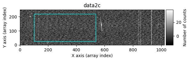
In this case, the region to be cleaned is shown as a cyan-colored rectangle.

The cr2images() function also accepts a maxsize parameter, which indicates the maximum number of pixels each detected cosmic ray should have (if the number of pixels exceeds this value, the potential cosmic ray is not cleaned).

Using Images with Extensions (CCDData Objects)

Since our FITS images have extensions, the best way to work with them is to read each one as an object of type CCDData, and proceed to clean the corresponding data arrays before saving the result in a new FITS file that preserves the extensions.

Cosmic ray cleaning will be reflected in the MASK extension (marking the replaced pixels) and in the UNCERT extension, which contains the uncertainty array (replacing with the uncertainties from the companion image).

We again start from the pair of images to be cleaned.

input_filename1 = 'ftdz_45243.fits'
input_filename2 = 'ftdz_45244.fits'

We generate two objects of type CCDData.

ccdimage1 = CCDData.read(input_filename1)
ccdimage2 = CCDData.read(input_filename2)

We duplicate the two objects to store the result of executing the cosmic ray cleaning.

ccdimage1_clean = ccdimage1.copy()
ccdimage2_clean = ccdimage2.copy()

Cleaning the Data Arrays

We perform cosmic ray cleaning only on the data arrays (i.e., the .data attributes of the CCDData objects), including the computation of the corresponding masks.

ioffx = 0
ioffy = -4
tsigma_peak = 10
tsigma_tail = 3

ccdimage1_clean.data, ccdimage2_clean.data, mask_data1c, mask_data2c = tea.cr2images(
    data1=ccdimage1.data,
    data2=ccdimage2.data,
    ioffx=ioffx,
    ioffy=ioffy,
    tsigma_peak=tsigma_peak,
    tsigma_tail=tsigma_tail,
    return_masks=True
)

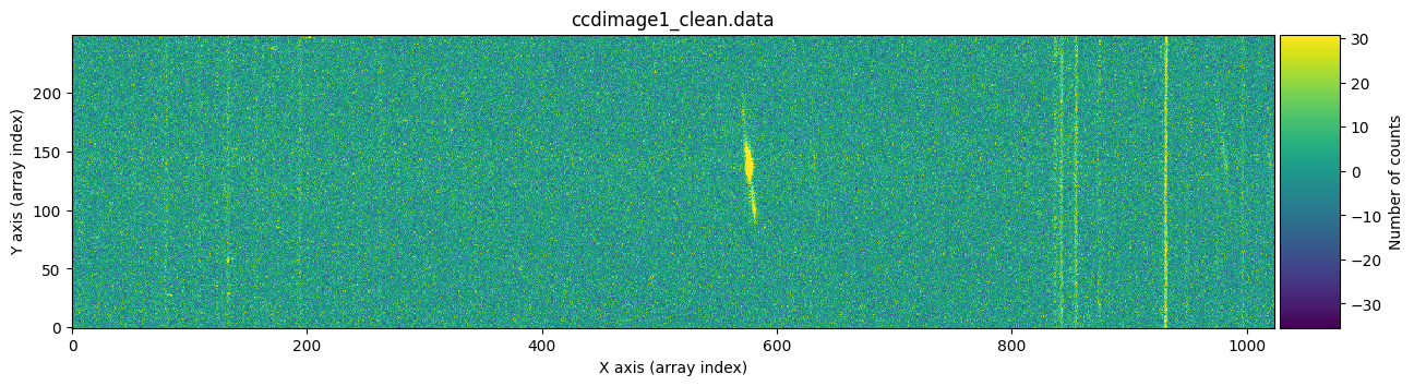
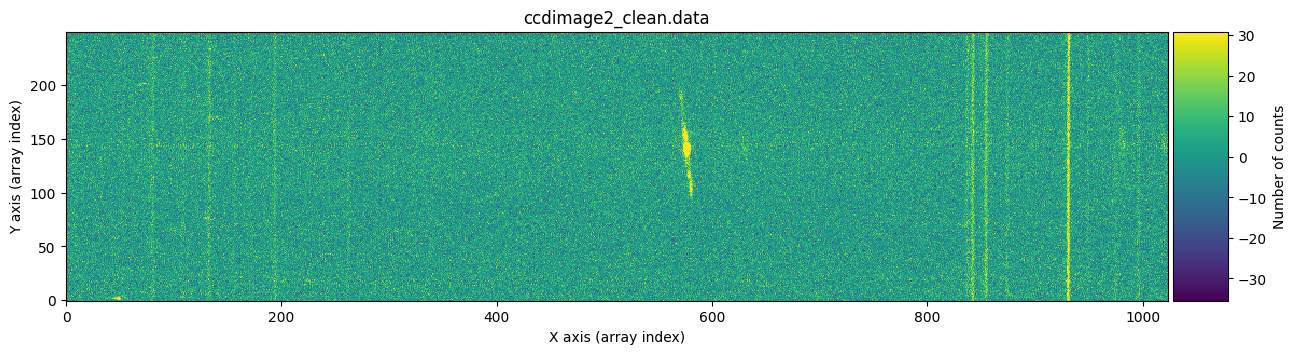
We visually verify that the stored images are free of cosmic rays.

vmin, vmax = np.percentile(ccdimage1_clean.data, [0, 99.9])

for dumdata, title in zip([ccdimage1_clean.data, ccdimage2_clean.data],
                          ['ccdimage1_clean.data', 'ccdimage2_clean.data']):
    fig, ax = plt.subplots(figsize=(15, 5))
    tea.imshow(fig, ax, dumdata, vmin=vmin, vmax=vmax)
    ax.set_title(title)
    plt.show()

Transferring Cleaned Pixels to the MASK Extension

We include in the masks of each image (i.e., the .mask attributes of the CCDData objects) the positions of the cosmic rays. We only modify the pixels indicated in the masks returned by cr2images() (in case the masks of the CCDData objects already have True values before reaching this point). Since the masks computed by cr2images() contain values 0 and 1, we convert them to boolean using .astype(bool).

ccdimage1_clean.mask[mask_data1c.astype(bool)] = True
ccdimage2_clean.mask[mask_data2c.astype(bool)] = True

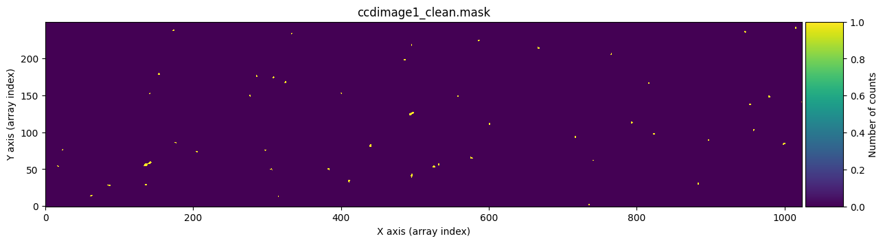
We check that it works by graphically comparing the calculated mask mask_data1c with the one stored in ccdimage1_clean.mask.

for dumdata, title in zip([mask_data1c, ccdimage1_clean.mask.astype(int)],
                          ['mask_data1c', 'ccdimage1_clean.mask']):
    fig, ax = plt.subplots(figsize=(15, 5))
    tea.imshow(fig, ax, dumdata, vmin=0, vmax=1)
    ax.set_title(title)
    plt.show()

Transferring the cleaned pixels to the UNCERT extension

For the uncertainty arrays, we insert into the first image the values from the second (before cleaning), and into the second the values from the first (before cleaning). Here we are assuming that there has been no cosmic ray coincidence, which we already know is something that did not happen in this particular pair of exposures.

ccdimage1_clean.uncertainty.array[ccdimage1_clean.mask] = \
    ccdimage2.uncertainty.array[ccdimage1_clean.mask]

ccdimage2_clean.uncertainty.array[ccdimage2_clean.mask] = \
    ccdimage1.uncertainty.array[ccdimage2_clean.mask]

We can check graphically whether this has worked by comparing, for example, the uncertainty arrays of the first exposure before and after cosmic ray cleaning.

vmin, vmax = np.percentile(ccdimage1.uncertainty.array, [0, 99.9])

for dumdata, title in zip([ccdimage1.uncertainty.array, ccdimage1_clean.uncertainty.array],
                          ['ccdimage1.uncertainty_array', 'ccdimage1_clean.uncertainty.array']):
    fig, ax = plt.subplots(figsize=(15, 5))
    tea.imshow(fig, ax, dumdata, vmin=vmin, vmax=vmax)
    ax.set_title(title)
    plt.show()

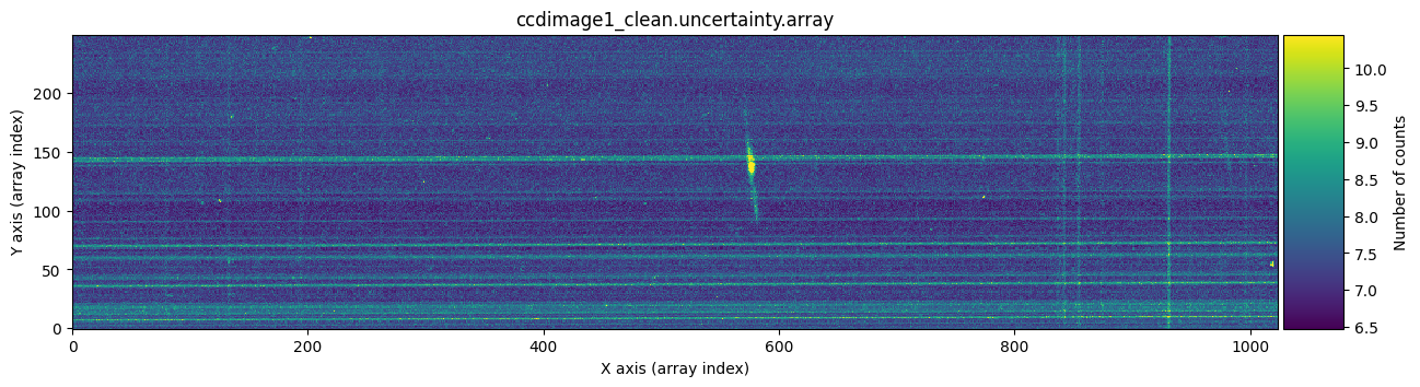
The bright horizontal lines correspond to the uncertainties introduced by the Flat Field (remember that the slit had defects). What’s important here is that we have been able to replace, in the uncertainty array, the information from another uncertainty array for the pixels affected by cosmic rays.

Saving the result

The final step is to save the result, including information in the headers to maintain traceability of the process carried out. The name of the output file is, in each case, the original name with the prefix c.

for input_filename, ccdimage_clean in zip([input_filename1, input_filename2],
                                          [ccdimage1_clean, ccdimage2_clean]):
    # update FILENAME keyword with output file name
    output_filename = f'c{input_filename}'
    ccdimage_clean.header['FILENAME'] = output_filename
    
    # update HISTORY in header
    ccdimage_clean.header['HISTORY'] = '-------------------'
    ccdimage_clean.header['HISTORY'] = f"{datetime.now().strftime('%Y-%m-%d %H:%M:%S')}"
    ccdimage_clean.header['HISTORY'] = 'using cr2images:'
    ccdimage_clean.header['HISTORY'] = f'- infile1: {Path(input_filename1).name}'
    ccdimage_clean.header['HISTORY'] = f'- infile2: {Path(input_filename2).name}'
    ccdimage_clean.header['HISTORY'] = f'- ioffx: {ioffx}'
    ccdimage_clean.header['HISTORY'] = f'- ioffy: {ioffy}'
    ccdimage_clean.header['HISTORY'] = f'- tsigma_peak: {tsigma_peak}'
    ccdimage_clean.header['HISTORY'] = f'- tsigma_tail: {tsigma_tail}'
        
    # save result
    ccdimage_clean.write(output_filename, overwrite='yes')
    print(f'Output file name: {output_filename}')

Output file name: cftdz_45243.fits
Output file name: cftdz_45244.fits

Auxiliary function apply_cr2images_ccddata()

To facilitate the handling of CCDData objects, we can use the auxiliary function apply_cr2images_ccddata(), designed to clean cosmic rays from pairs of images by directly specifying the names of the input and output FITS files (as well as the specific parameters of the cr2images() function corresponding to the cosmic ray detection strategy).

For example, to clean the pair of images we just used a moment ago, it is enough to run:

tea.apply_cr2images_ccddata(
    infile1=input_filename1,
    infile2=input_filename2,
    outfile1=f'cc{input_filename1}',
    outfile2=f'cc{input_filename2}',
    ioffx=ioffx,
    ioffy=ioffy,
    tsigma_peak=tsigma_peak,
    tsigma_tail=tsigma_tail
)

Output file name: ccftdz_45243.fits
Output file name: ccftdz_45244.fits

The images cftdz_45243.fits and ccftdz_45243.fits are identical. The same applies to cftdz_45244.fits and ccftdz_45244.fits.

What happens inside cr2images()?

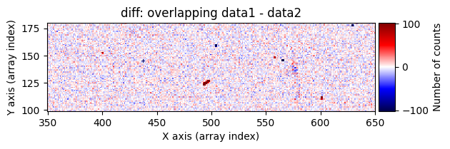
We can ask the cr2images() function to show us more information about what is happening during its execution. To do this, we use the debug_level parameter, which can take the values 0 (no additional information is shown), 1 (images before and after cleaning are shown), and 2 (a data histogram and the intermediate masks calculated are also shown). For example, using debug_level=1 will display the indices of the arrays corresponding to the overlapping region between the two images and the following images:

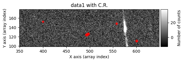
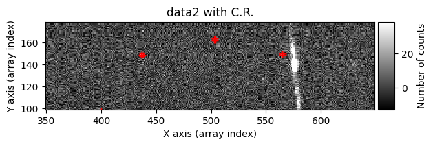
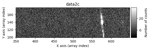
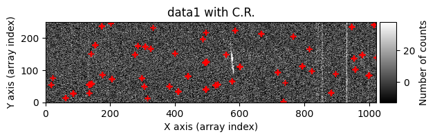
• data1: initial image number 1

• data1 with C.R.: initial image number 1, with the pixels to be corrected due to cosmic ray impact marked with red crosses

• data1c: initial image number 1 after cosmic ray removal

• data2: initial image number 2

• data2 with C.R.: initial image number 2, with the pixels to be corrected due to cosmic ray impact marked with red crosses

• data2c: initial image number 2 after cosmic ray removal

data1c, data2c, mask_data1c, mask_data2c = tea.cr2images(
    data1=data1,
    data2=data2,
    ioffx=0,
    ioffy=-4,
    tsigma_peak=10,
    tsigma_tail=3,
    return_masks=True,
    debug_level=1
)

Computing overlaping rectangle:
ioffx: 0
ioffx: -4
data1:  i1,  i2,  j1,  j2: 0, 246, 0, 1024
data2: ii1, ii2, jj1, jj2: 4, 250, 0, 1024
shape1: (246, 1024), shape2: (246, 1024), shape(diff): (246, 1024)

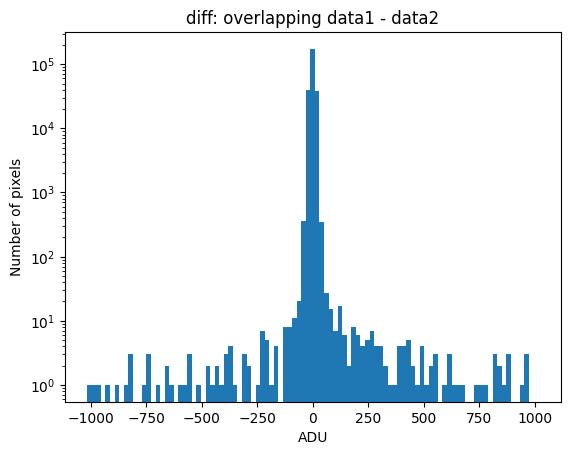
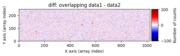
>>> Statistical summary of diff = overlapping data1 - data2:
>>> Median....: -0.179
>>> Robust_std: 10.149
>>> Searching for positive peaks (CR in data1) with tsigma_peak=10
>>> Found 52 positive peaks
>>> Searching for positive tails (CR in data1) with tsigma_tail=3
>>> Found 371 positive tails
>>> Merging positive peaks and tails
>>> Replacing 280 pixels affected by cosmic rays in data1
>>> Finished replacing pixels affected by cosmic rays in data1
>>> Searching for negative peaks (CR in data2) with tsigma_peak=10
>>> Found 31 negative peaks
>>> Searching for negative tails (CR in data2) with tsigma_tail=3
>>> Found 405 negative tails
>>> Merging negative peaks and tails
>>> Replacing 175 pixels affected by cosmic rays in data2
>>> Finished replacing pixels affected by cosmic rays in data2
Number of CR in data1: 52 peaks, 371 tails

Number of CR in data2: 31 peaks, 405 tails

Using debug_level=2, the indices of the arrays corresponding to the overlapping region between the two images will be displayed, along with a histogram and a representation of the diff image, as well as the following arrays:

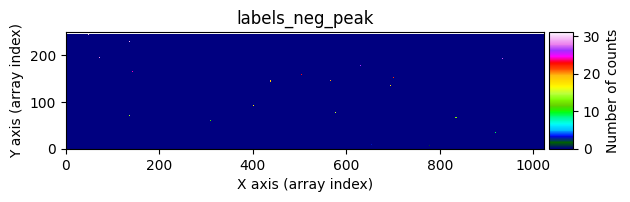
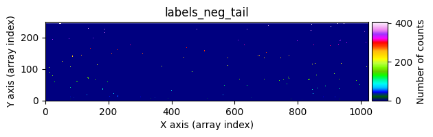
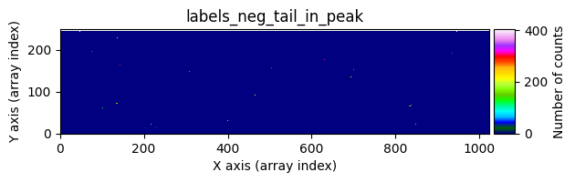
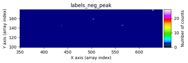
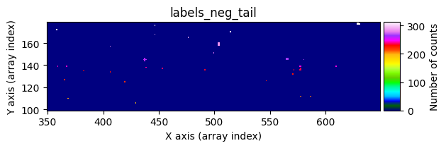
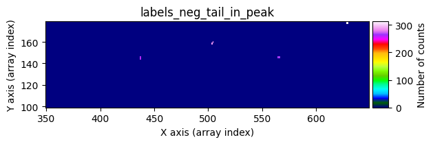
• data1: initial image number 1

• labels_pos_peak: image with labels of the peaks of the cosmic rays detected in data1

• labels_pos_tail: image with labels of the tails of the cosmic rays detected in data1

• labels_pos_tail_in_peak: labels of the cosmic rays in labels_pos_tail that appear in labels_pos_peak

• data1 with C.R.: initial image number 1, with the pixels to be corrected due to cosmic ray impact marked with red crosses

• data1c: initial image number 1 after cosmic ray removal

• data2: initial image number 2

• labels_neg_peak: image with labels of the peaks of the cosmic rays detected in data2

• labels_neg_tail: image with labels of the tails of the cosmic rays detected in data2

• labels_neg_tail_in_peak: labels of the cosmic rays in labels_neg_tail that appear in labels_neg_peak

• data2 with C.R.: initial image number 2, with the pixels to be corrected due to cosmic ray impact marked with red crosses

• data2c: initial image number 2 after cosmic ray removal

data1c, data2c, mask_data1c, mask_data2c = tea.cr2images(
    data1=data1,
    data2=data2,
    ioffx=0,
    ioffy=-4,
    tsigma_peak=10,
    tsigma_tail=3,
    return_masks=True,
    debug_level=2
)

Computing overlaping rectangle:
ioffx: 0
ioffx: -4
data1:  i1,  i2,  j1,  j2: 0, 246, 0, 1024
data2: ii1, ii2, jj1, jj2: 4, 250, 0, 1024
shape1: (246, 1024), shape2: (246, 1024), shape(diff): (246, 1024)

>>> Statistical summary of diff = overlapping data1 - data2:
>>> Median....: -0.179
>>> Robust_std: 10.149
>>> Searching for positive peaks (CR in data1) with tsigma_peak=10
>>> Found 52 positive peaks
>>> Searching for positive tails (CR in data1) with tsigma_tail=3
>>> Found 371 positive tails
>>> Merging positive peaks and tails
>>> Replacing 280 pixels affected by cosmic rays in data1
>>> Finished replacing pixels affected by cosmic rays in data1
>>> Searching for negative peaks (CR in data2) with tsigma_peak=10
>>> Found 31 negative peaks
>>> Searching for negative tails (CR in data2) with tsigma_tail=3
>>> Found 405 negative tails
>>> Merging negative peaks and tails
>>> Replacing 175 pixels affected by cosmic rays in data2
>>> Finished replacing pixels affected by cosmic rays in data2

Number of CR in data1: 52 peaks, 371 tails

Number of CR in data2: 31 peaks, 405 tails

We can repeat the previous command indicating that we want to visualize a zoom in a specific region. To do this, we must use the zoom_region_imshow parameter, which must be an object of type SliceRegion2D.

data1c, data2c, mask_data1c, mask_data2c = tea.cr2images(
    data1=data1,
    data2=data2,
    ioffx=0,
    ioffy=-4,
    tsigma_peak=10,
    tsigma_tail=3,
    return_masks=True,
    debug_level=2,
    zoom_region_imshow=tea.SliceRegion2D(np.s_[350:650, 100:180], mode='fits')
)

Computing overlaping rectangle:
ioffx: 0
ioffx: -4
data1:  i1,  i2,  j1,  j2: 0, 246, 0, 1024
data2: ii1, ii2, jj1, jj2: 4, 250, 0, 1024
shape1: (246, 1024), shape2: (246, 1024), shape(diff): (246, 1024)

>>> Statistical summary of diff = overlapping data1 - data2:
>>> Median....: -0.179
>>> Robust_std: 10.149
>>> Searching for positive peaks (CR in data1) with tsigma_peak=10
>>> Found 52 positive peaks
>>> Searching for positive tails (CR in data1) with tsigma_tail=3
>>> Found 371 positive tails
>>> Merging positive peaks and tails
>>> Replacing 280 pixels affected by cosmic rays in data1
>>> Finished replacing pixels affected by cosmic rays in data1
>>> Searching for negative peaks (CR in data2) with tsigma_peak=10
>>> Found 31 negative peaks
>>> Searching for negative tails (CR in data2) with tsigma_tail=3
>>> Found 405 negative tails
>>> Merging negative peaks and tails
>>> Replacing 175 pixels affected by cosmic rays in data2
>>> Finished replacing pixels affected by cosmic rays in data2

Number of CR in data1: 52 peaks, 371 tails

Number of CR in data2: 31 peaks, 405 tails

Cleaning individual exposures

We can also use the cr2images() function to attempt cosmic ray removal even in situations where we only have a single exposure. In that case, we can ask cr2images() to generate a fictitious image number 2 from the only available image. This is done using a median filter (in 2 dimensions), with a kernel of the dimensions specified by the median_size tuple. Note that in this case data2 is not used in the function call (and it also makes no sense to specify ioffx, ioffy). Internally, cr2images() makes a call to scipy.ndimage.median_filter(data1, size=median_size) to generate data2. Obviously, we can generate a data2 array independently before calling cr2images() and not use median_size.

median_size = (9, 3)  # kernel size in the (Y-axis, X-axis), following the Python convention
tsigma_peak = 10
tsigma_tail = 3

data1c, data2c, mask_data1c, mask_data2c = tea.cr2images(
    data1=data1,
    median_size=median_size,
    tsigma_peak=tsigma_peak,
    tsigma_tail=tsigma_tail,
    return_masks=True,
    debug_level=1,
    zoom_region_imshow=tea.SliceRegion2D(np.s_[350:650, 100:180], mode='fits')
)

Computing overlaping rectangle:
ioffx: 0
ioffx: 0
data1:  i1,  i2,  j1,  j2: 0, 250, 0, 1024
data2: ii1, ii2, jj1, jj2: 0, 250, 0, 1024
shape1: (250, 1024), shape2: (250, 1024), shape(diff): (250, 1024)

>>> Statistical summary of diff = overlapping data1 - data2:
>>> Median....: 0.000
>>> Robust_std: 6.942
>>> Searching for positive peaks (CR in data1) with tsigma_peak=10
>>> Found 53 positive peaks
>>> Searching for positive tails (CR in data1) with tsigma_tail=3
>>> Found 699 positive tails
>>> Merging positive peaks and tails
>>> Replacing 297 pixels affected by cosmic rays in data1
>>> Finished replacing pixels affected by cosmic rays in data1
Number of CR in data1: 53 peaks, 699 tails

In this case, the cleaning is not perfect: some pixels affected by cosmic rays still remain. It’s not easy for this method to do a perfect job. On one hand, increasing median_size can help remove cosmic rays more effectively in the fictitious image data2, but this comes at the cost of smoothing the information in image data1, and it’s possible that signal corresponding to real image data may be mistakenly detected as a cosmic ray. On the other hand, the signal of the pixels detected as cosmic rays is replaced by the smoothed fictitious image data2, so if the original cosmic ray is large and median_size is smaller, the correction will not be good.

The best strategy, then, is to try different values of median_size through trial and error.

In this case, it is also possible to use the auxiliary function apply_cr2images_ccddata() to directly clean a FITS image that stores the information of a CCDData object. Since only one image is used, the pixels affected by cosmic rays in the array stored in the UNCERT extension are replaced by the smoothed version of the UNCERT array from the initial image.

tea.apply_cr2images_ccddata(
    infile1=input_filename1,
    outfile1=f'ccc{input_filename1}',
    median_size=median_size,
    tsigma_peak=tsigma_peak,
    tsigma_tail=tsigma_tail,
    debug_level=1
)

Computing overlaping rectangle:
ioffx: 0
ioffx: 0
data1:  i1,  i2,  j1,  j2: 0, 250, 0, 1024
data2: ii1, ii2, jj1, jj2: 0, 250, 0, 1024
shape1: (250, 1024), shape2: (250, 1024), shape(diff): (250, 1024)

>>> Statistical summary of diff = overlapping data1 - data2:
>>> Median....: 0.000
>>> Robust_std: 6.942
>>> Searching for positive peaks (CR in data1) with tsigma_peak=10
>>> Found 53 positive peaks
>>> Searching for positive tails (CR in data1) with tsigma_tail=3
>>> Found 699 positive tails
>>> Merging positive peaks and tails
>>> Replacing 297 pixels affected by cosmic rays in data1
>>> Finished replacing pixels affected by cosmic rays in data1
Number of CR in data1: 53 peaks, 699 tails

Output file name: cccftdz_45243.fits

time_end = datetime.now()
tea.elapsed_time(time_ini, time_end)

system...........: Linux
release..........: 6.11.0-1018-azure
machine..........: x86_64
node.............: runnervmymu0l
Python executable: /opt/hostedtoolcache/Python/3.12.12/x64/bin/python
teareduce version: 0.6.9
Initial time.....: 2026-01-27 04:39:35.291492
Final time.......: 2026-01-27 04:39:50.661743
Elapsed time.....: 0:00:15.370251